This blog is based on the course (CMU Databases Systems / Fall 2019) provided by Prof. Andy Pavlo and the course notes.

General
- Basic Terms
- Relational Algebra
Storage Management
Buffer Management
- Locks vs. Latches
- Buffer Pool
Access Methods
Operator Execution
Query Execution
Query Parallism
Query Planning & Optimization
- Rule-based Query Optimization
- Cost-based Query Optimization
Transactions
Recovery

1. General

A database is an organized collection of inter-related data that models some aspect of the real-world. A database management system (DBMS) is the software that manages a database, which allows applications to store and analyze information in a database. A general-purpose DBMS is designed to allow the definition, creation, querying, update, and administration of databases.

1.1 Basic Terms

	Description
Data Model	A data model is collection of concepts for describing the data in a database, some examples are, for most DBMSs: relational; for NoSQL: key/value, graph, document, column-family; for maching learning: array/matrix.
Schema	A schema is a description of a particular collection of data, using a given data model.
Relation	A relation is unordered set that contain that relationship of attributes that represent entities. n-ary relation = table with n columns.
Tuple	A tuple is a set of attribute values (also known as its domain) in the relation.
Primary Key	A relation's primiary key uniquely identifies a single tuple. Some DBMSs automatically create an internal primary key if users don't define one.
Foreign Key	A foreign key specifies that an attribute from one relation has to map to a tuple in another relation.
Nested Query	Queries containing other queries, they are often difficult to optimize. Many modern DBMSs will try to rewrite the nested queries using join operators.
Common Table Expressions	Provides a way to write auxiliary statements for use in a larger query. Essentially, it like a temp table just for one query.

1.2 Relational Algebra

Fundamental operations to retrieve and manipulate tuples in a relation. Each operator takes one or more relations as its inputs and outputs a new relation. Widely-used ones are: select, projecton, union, intersection, difference, product, and join.

Select: choose a subset of the tuples from a relation that satisfies a selection predicte. [operation on rows in tables]
Projection: generate a relation with tuples that contains only the specified attributes. [operation on columns in tables]
Union: generate a relation that contains all tuples that appear in either only one or both input relations.
Intersection: generate a relation that contains only the tuples that appear in both of the input relations.
Difference: generate a relation that contains only the tuples that appear in the first and not the second of the input relations.
Product: generate a relation that contains all possible combinations of tuples from the input relations.
(Natural) Join: generate a relation that contains all tuples that are a combination of two tuples (one from each input relation) with a common value(s) for one or more attributes.

2. Storage Management

We will focus on a “disk-oriented” DBMS architecture that assumes that primary storage location of the database is on non-volatile disk. At the top of the storage hierarchy you have the devices that are closest to the CPU. This is the fastest storage but it is also the smallest and most expensive. The further you get away from the CPU, the storage devices have larger the capacities but are much slower and farther away from the CPU. These devices also get cheaper per GB.

Why use DBMS instead of OS: DBMS (almost) always wants to control things itself and can do a better job at it, such as flushing dirty pages to disk in the correct order, specialized prefetching, buffer replacement policy, thread/process scheduling.

File Storage: The DBMS stores a database as one or more files on disk. The OS know nothing about the contents of these files.

Storage Manager: The DBMS’s storage manager is responsible for managing a database’s files. It represents the files as a collection of pages. It also keeps track of what data has been read and written to pages, as well how much free space there is in the pages.

2.1 Database Page

A page is a fixed-size block of data. It can contain tuples, meta-data, indexes, log records, etc. Most systems don’t mix page types, for exmaple, a page only for tuples, the other page only for log records, another page is only for indexes. Some systems require a page to be self-contained. Each page is given a unique identifier. The DBMS uses an indirection layer to map page ids to physical locations.

There are three different notions of “pages” in a DBMS:

Hardware Page (usually 4KB), the level guarantees an atomic write of the size of the hardware page.
OS Page (usually 4K).
Database Page (usually 512B-16KB).

Different DBMSs manage pages in files on disk in different ways:

Heap File Organization.
Sequential / Sorted File Organization.
Hashing File Organization.

2.2 Page Layout

Every page includes a header that records meta-data about the page’s contents: (1) Page size, (2) Checksum, (3) DBMS version, (4) Transaction visibility, (5) Some systems require pages to be self-contained (e.g Oracle).

There are two main approaches to laying out data in pages: (1) slotted-pages and (2) log-structured.

Slotted Pages: Page maps slots to offsets

Most common approach used in DBMSs today.
Header keeps track of the number of used slots and the offset of the starting location of last used slot and a slot array, which keeps track of the location of the start of each tuple.
To add a tuple, the slot array will grow from the beginning to the end, and the data of the tuples will grow from end to the beginning. The page is considered full when the slot array and the tuple data meet.

Log-Structured: Instead of storing tuples, the DBMS only stores log records

Stores records to file of how the database was modified (insert, update, deletes).
To read a record, the DBMS scans the log file backwards and "recreates" the tuple.
Fast writes, potentially slow reads.
Works well on append-only storage because the DBMS cannot go back and update the data.
To avoid long reads the DBMS can have indexes to allow it to jump to specific locations in the log. It can also periodically compact the log (if it had a tuple and then made an update to it, it could compact it down to just inserting the updated tuple). The issue with compaction is the DBMS ends up with write amplification (it re-writs the same data over and over again).

2.3 Database Heap

A heap file is an unordered collection of pages where tuples are stored in random order. The DBMS can locate a page on disk given a page id by using a linked list of pages or a page directory.

Linked List: Header page holds pointers to to a list of free pages and a list of data pages. However, if the DBMS is looking for a specific page, it has to do a sequential scan on the data page list until it finds the page it is looking for.
Page Directory: DBMS maintains special pages that track locations of data pages along with the amount of free space on each page.

2.4 Data Representation

A data representation scheme is how a DBMS stores the bytes for a value. There are five main types that can be stored in tuples: integers, variable precision numbers, fixed point precision numbers, variable length values, and dates/times.

Integers:

Most DBMSs store integers using their "native" C/C++ types as specified by the IEEE-754 standard. These values are fixed length.
Examples: INTEGER, BIGINT, SMALLINT, TINYINT.

Variable Precision Numbers:

Inexact, variable-precision numeric type that uses the "native" C/C++ types specified by IEEE-754 standard. These values are also fixed length.
Variable-precision numbers are faster to compute than arbitrary precision numbers because the CPU can execute instructions on them directly.
Examples: FLOAT, REAL.

Fixed Point Precision Numbers

These are numeric data types with arbitrary precision and scale. They are typically stored in exact, variable-length binary representation with additional meta-data that will tell the system things like where the decimal should be.
These data types are used when rounding errors are unacceptable, but the DBMS pays a performance penalty to get this accuracy.
Example: NUMERIC, DECIMAL.

Variable Length Data

An array of bytes of arbitrary length.
Has a header that keeps track of the length of the string to make it easy to jump to the next value.
Most DBMSs do not allow a tuple to exceed the size of a single page, so they solve this issue by writing the value on an overflow page and have the tuple contain a reference to that page.
Some systems will let you store these large values in an external file, and then the tuple will contain a pointer to that file. For example, if our database is storing photo information, we can store the photos in the external files rather than having them take up large amounts of space in the DBMS. One downside of this is that the DBMS cannot manipulate the contents of this file.
Example: VARCHAR, VARBINARY, TEXT, BLOB.

Dates and Times

Usually, these are represented as the number of (micro/milli) seconds since the unix epoch.
Example: TIME, DATE, TIMESTAMP.

2.5 Workloads

OLTP: On-line Transaction Processing

Fast, short running operations
Queries operate on single entity at a time
More writes than reads
Repetitive operations
Usually the kind of application that people build first
Example: User invocations of Amazon. They can add things to their cart, they can make purchases, but the actions only affect their account

OLAP: On-line Analyitical Processing

Long running, more complex queries
Reads large portions of the database
Exploratory queries
Deriving new data from data collected on the OLTP side
Example: Compute the five most bought items over a one month period for these geographical locations

2.6 Storage Models

N-Ary Storage Model (NSM), aka Row-Store

The DBMS stores all of the attributes for a single tuple contiguously, so NSM is also known as a “row store.” This approach is ideal for OLTP workloads where transactions tend to operate only an individual entity and insert heavy workloads. It is ideal because it takes only one fetch to be able to get all of the attributes for a single tuple.

Decomposition Storage Model (DSM), aka Column-Store

The DBMS stores a single attribute (column) for all tuples contiguously in a block of data. Also known as a “column store.” This model is ideal for OLAP workloads where read-only queries perform large scans over a subset of the table’s attributes.

3. Buffer Management

3.1 Locks vs. Latches

Locks

Protect the database logical contents (e.g., tuples, tables, databases) from other transactions.
Held for transaction duration.
Need to be able to rollback changes

Latches

Protects the critical sections of the DBMS’s internal data structures from other threads.
Held for operation duration.
Do not need to be able to rollback changes.

	Locks	Latches
Separate...	User Transaction	Threads
Protect...	Database Contents	In-Memory Data Strctures
During...	Entire Transactions	Critical Sections
Modes...	Shared, Exclusive, Update, Intention	Read, Write
Deadlock	Detection & Resolution	Avoidance
...by...	Waits-for, Timeout, Aborts	Coding Discipline
Kept in...	Lock Manager	Protected Data Structures

3.2 Buffer Pool

A buffer pool is an area of main memory that has been allocated by the database manager for the purpose of caching table and index data as it is read from disk. It is a region of memory organized as an array of fixed size pages. Each array entry is called a memory page or frame. When the DBMS requests a page, an exact copy is placed into one of these frames.

Meta-data maintained by the buffer pool

Page Table: In-memory hash table that keeps track of pages that are currently in memory. It maps page ids to frame locations in the buffer pool.

Dirty-flag: Threads set this flag when it modifies a page. This indicates to storage manager that the page must be written back to disk.

Pin Counter: This tracks the number of threads that are currently accessing that page (either reading or modifying it). A thread has to increment the counter before they access the page. If a page’s count is greater than zero, then the storage manager is not allowed to evict that page from memory.

Optimizations

Multiple Buffer Pools: The DBMS can also have multiple buffer pools for different purposes. This helps reduce latch contention and improves locality.
Pre-Fetching: The DBMS can also optimize by pre-fetching pages based on the query plan. Commonly done when accessing pages sequentially.
Scan Sharing: Query cursors can attach to other cursors and scan pages together.

Allocation Policies

Global Policies: How a DBMS should make decisions for all active txns.
Local Policies: Allocate frames to a specific txn without considering the behavior of concurrent txns.

4. Access Methods

Access methods are about how to support the DBMS’s execution engine to read/write data from pages.

A DBMS uses various data structures for many different parts of the system internals:

Internal Meta-Data: Keep track of information about the database and the system state.
Core Data Storage: Can be used as the base storage for tuples in the database.
Temporary Data Structures: The DBMS can build data structures on the fly while processing a query to speed up execution (e.g., hash tables for joins).
Table Indexes: Auxiliary data structures to make it easier to find specific tuples.

4.1 Hash Tables

A hash table implements an associative array abstract data type that maps keys to values. It provides on average $O(1)$ operation complexity and $O(n)$ storage complexity.

A hash table implementation is comprised of two parts:

Hash Function: How to map a large key space into a smaller domain. This is used to compute an index into an array of buckets or slots. Need to consider the trade-off between fast execution vs. collision rate.
Hashing Scheme: How to handle key collisions after hashing. Need to consider the trade-off between the need to allocate a large hash table to reduce collisions vs. executing additional instructions to find/insert keys.

4.1.1 Hash Functions

A hash function takes in any key as its input. It then return an integer representation of that key (i.e., the “hash”). The function’s output is deterministic (i.e., the same key should always generate the same hash output).

The current state-of-the-art hash function is Facebook XXHash3

4.1.2 Static Hashing Schemes

A static hashing scheme is one where the size of the hash table is fixed. This means that if the DBMS runs out of storage space in the hash table, then it has to rebuild it from scratch with a larger table. Typically the new hash table is twice the size of the original hash table.

Linear Probe Hashing

This is the most basic hashing scheme. It is also typically the fastest. It uses a single table of slots. The hash function allows the DBMS to quickly jump to slots and look for the desired key.

Resolve collisions by linearly searching for the next free slot in the table.
To see if value is present, go to slot using hash, and scan for the key. The scan stops if you find the desired key or you encounter an empty slot.

Robin Hood Hashing This is an extension of linear probe hashing that seeks to reduce the maximum distance of each key from their optimal position in the hash table. Allows threads to steal slots from “rich” keys and give them to “poor” keys.

Each key tracks the number of positions they are from where its optimal position in the table.
On insert, a key takes the slot of another key if the first key is farther away from its optimal position than the second key. The removed key then has to be re-inserted back into the table.

Cuckoo Hashing Instead of using a single hash table, this approach maintains multiple (usually 2-3) hash tables with different hash functions. The hash function are the same algorithm (e.g., XXHash, CityHash); they generate different hashes for the same key by using different seed values.

On insert, check every table and pick anyone that has a free slot.
If no table has free slot, evict element from one of them, and rehash it to find a new location.
If we find a cycle, then we can rebuild all of the hash tables with new hash function seeds (less common) or rebuild the hash tables using larger tables (more common).

4.1.3 Dynamic Hashing Schemes

Dynamic hashing schemes are able to resize the hash table on demand without needing to rebuild the entire table. The schemes perform this resizing in different ways that can either maximize reads or writes

Chained Hashing This is the most common dynamic hashing scheme. The DBMS maintains a linked list of buckets for each slot in the hash table.

Resolves collisions by placing elements with same hash key into the same bucket.
If bucket is full, add another bucket to that chain. The hash table can grow infinitely because the DBMS keeps adding new buckets.

Extendible Hashing Improved variant of chained hashing that splits buckets instead of letting chains to grow forever. The core idea behind re-balancing the hash table is to to move bucket entries on split and increase the number of bits to examine to find entries in the hash table. This means that the DBMS only has to move data within the buckets of the split chain; all other buckets are left untouched

The DBMS maintains a global and local depth bit counts that determine the number bits needed to find buckets in the slot array.
When a bucket is full, the DBMS splits the bucket and reshuffle its elements. If the local depth of the split bucket is less than the global depth, then the new bucket is just added to the existing slot array. Otherwise, the DBMS doubles the size of the slot array to accommodate the new bucket and increments the global depth counter.

4.2 Tree Indexes

A table index is a replica of a subset of a table’s columns that is organized in such a way that allows the DBMS to find tuples more quickly than performing a sequential scan. The DBMS ensures that the contents of the tables and the indexes are always in sync.

It is the DBMS’s job to figure out the best indexes to use to execute queries. There is a trade-off on the number of indexes to create per database (indexes use storage and require maintenance).

4.2.1 B+ Tree Introduction

A B+ Tree is a self-balancing tree data structure that keeps data sorted and allows searches, sequential access, insertion, and deletions in $O(log(n))$. It is optimized for disk-oriented DBMSs that read/write large blocks of data. Almost every modern DBMS that supports order-preserving indexes uses a B+ Tree.

The inner node keys in a B+ Tree cannot tell you whether a key exists in the index. You must always traverse to the leaf node. This means that you could have (at least) one buffer pool page miss per level in the tree just to find out a key does not exist.

Almost every modern DBMS that supports order-preserving indexes uses a B+ Tree.

It is perfectly balanced (i.e., every leaf node is at the same depth).
Every inner node other than the root is at least half full ($M/2 - 1 <=$ num of keys $<= M - 1$).
Every inner node with $k$ keys has $k+1$ non-null children.
The max degree of a B+ tree is the number of values a node can has at most plus one, i.e., the number of links to their children.

Every node in a B+ Tree contains an array of key/value pairs:

Arrays at every node are (almost) sorted by the keys.
The value array for inner nodes will contain pointers to other nodes.
Two approaches for leaf node values:

Record IDs: A pointer to the location of the tuple
Tuple Data: The actual contents of the tuple is stored in the leaf node

Insertion

Find correct leaf $L$.
Add new entry into L in sorted order:

If $L$ has enough space, the operation done.
Otherwise split $L$ into two nodes $L$ and $L_2$. Redistribute entries evenly and copy up middle key. Insert index entry pointing to $L_2$ into parent of $L$.

To split an inner node, redistribute entries evenly, but push up the middle key.

Deletion

Find correct leaf $L$.
Remove the entry:

If $L$ is at least half full, the operation is done.
Otherwise, you can try to redistribute, borrowing from sibling.
If redistribution fails, merge $L$ and sibling.

If merge occurred, you must delete entry in parent pointing to $L$.

4.2.2 B+ Tree Design Decisions

Node Size

The optimal node size for a B+Tree depends on the speed of the disk. The idea is to amortize the cost of reading a node from disk into memory over as many key/value pairs as possible
The slower the disk, then the larger the idea node size.
Some workloads may be more scan-heavy versus having more single key look-ups.

Merge Threshold

Some DBMS do not always merge when it's half full.
Delaying a merge operation may reduce the amount of reorganization.
It may be better for the DBMS to let underflows to occur and then periodically rebuild the entire tree to re-balance it.

Variable Length keys

Pointers: Store keys as pointers to the tuples attribute (very rarely used).
Variable-length Nodes: The size of each node in the B+ Tree can vary, but requires careful memory management. This approach is also rare.
Key Map / Indirection: Embed an array of pointers that map to the key+value list within the node. This is similar to slotted pages discussed before. This is the most common approach.

Non-Unique Indexes

Duplicate Keys: Use the same leaf node layout but store duplicate keys multiple times.
Value Lists: Store each key only once and maintain a linked list of unique values.

Intra-Node Search

Linear: Scan the key/value entries in the node from beginning to end. Stop when you find the key that you are looking for. This does not require the key/value entries to be pre-sorted.
Binary: Jump to the middle key, and then pivot left/right depending on whether that middle key is less than or greater than the search key. This requires the key/value entries to be pre-sorted.
Interpolation: Approximate the starting location of the search key based on the known low/high key values in the node. Then perform linear scan from that location. This requires the key/value entries to be pre-sorted.

4.2.3 B+ Tree Optimizations

Prefix Compression

Sorted keys in the same leaf node are likely to have the same prefix.
Instead of storing the entire key each time, extract common prefix and store only unique suffix for each key.

Suffix Truncation

The keys in the inner nodes are only used to "direct traffic", we do not need the entire key.
Store a minimum prefix that is needed to correctly route probes into the index.

Bulk Inserts

The fastest way to build a B+ Tree from scratch is to first sort the keys and then build the index from the bottom up.
This will be faster than inserting one-by-one since there are no splits or merges.

Pointer Swizzling

Nodes use page ids to reference other nodes in the index. The DBMS must get the memory location from the page table during traversal.
If a page is pinned in the buffer pool, then we can store raw pointers instead of page ids. This avoids address lookups from the page table.

4.3 Additional Index Usage

Implicit Indexes: Most DBMSs will automatically create an index to enforce integrity constraints (e.g., primary keys, unique constraints).

Partial Indexes: Create an index on a subset of the entire table. This potentially reduces size and the amount of overhead to maintain it. One common use case is to partition indexes by date ranges, i.e., create a separate index per month, year.

Covering Indexes: All attributes needed to process the query are available in an index, then the DBMS does not need to retrieve the tuple. The DBMS can complete the entire query just based on the data available in the index. This reduces contention on the DBMS’s buffer pool resources.

Index Include Columns: Embed additional columns in index to support index-only queries.

Function/Expression Indexes: Store the output of a function or expression as the key instead of the original value. It is the DBMS’s job to recognize which queries can use that index.

4.3.1 Radix Tree

A radix tree is a variant of a trie data structure. It uses digital representation of keys to examine prefixes one-by-one instead of comparing entire key. It is different than a trie in that there is not a node for each element in key, nodes are consolidated to represent the largest prefix before keys differ.

The height of tree depends on the length of keys and not the number of keys like in a B+ Tree. The path to a leaf nodes represents the key of the leaf. Not all attribute types can be decomposed into binary comparable digits for a radix tree

4.3.2 Inverted Indexes

An inverted index stores a mapping of words to records that contain those words in the target attribute. These are sometimes called a full-text search indexes in DBMSs.

Most of the major DBMSs support inverted indexes natively, but there are specialized DBMSs where this is the only table index data structure available.

Query Types:

Phrase Searches: Find records that contain a list of words in the given order.
Proximity Searches: Find records where two words occur within n words of each other.
Wildcard Searches: Find records that contain words that match some pattern (e.g., regular expression).

Design Decisions:

What To Store: The index needs to store at least the words contained in each record (separated by punctuation characters). It can also include additional information such as the word frequency, position, and other meta-data.
When To Update: Updating an inverted index every time the table is modified is expensive and slow. Thus, most DBMSs will maintain auxiliary data structures to "stage" updates and then update the index in batches.

4.4 Concurrency Control Indexes

A concurrency control protocol is the method that the DBMS uses to ensure “correct” results for concurrent operations on a shared object.

A protocol’s correctness criteria can vary:

Logical Correctness: Can I see the data that I am supposed to see? This means that the thread is able to read values that it should be allowed to read.
Physical Correctness: Is the internal representation of the object sound? This means that there are not pointers in our data structure that will cause a thread to read invalid memory locations.

4.4.1 Latch Implementations

The underlying primitive that we can use to implement a latch is through an atomic compare-and-swap (CAS) instruction that modern CPUs provide. With this, a thread can check the contents of a memory location to see whether it has a certain value. If it does, then the CPU will swap the old value with a new one. Otherwise the memory location remains unmodified.

There are several approaches to implementing a latch in a DBMS, as shown in following. Each approach have different tradeoffs in terms of engineering complexity and runtime performance. These test-and-set steps are performed atomically (i.e., no other thread can update the value after one thread checks it but before it updates it).

Blocking OS Mutex

Use the OS built-in mutex infrastructure as a latch. The futex (fast user-space mutex) is comprised of (1) a spin latch in user-space and (2) a OS-level mutex. If the DBMS can acquire the user-space latch, then the latch is set. It appears as a single latch to the DBMS even though it contains two internal latches. If the DBMS fails to acquire the user-space latch, then it goes down into the kernel and tries to acquire a more expensive mutex. If the DBMS fails to acquire this second mutex, then the thread notifies the OS that it is blocked on the lock and then it is descheduled.

OS mutex is generally a bad idea inside of DBMSs as it is managed by OS and has large overhead.

Example: std::mutex
Advantages: Simple to use and requires no additional coding in DBMS.
Disadvantages: Expensive and non-scalable (about 25 ns per lock/unlock invocation) because of OS scheduling.

Test-and-Set Spin Latch (TAS)

Spin latches are a more efficient alternative to an OS mutex as it is controlled by the DBMSs. A spin latch is essentially a location in memory that threads try to update (e.g., setting a boolean value to true). A thread performs CAS to attempt to update the memory location. If it cannot, then it spins in a while loop forever trying to update it.

Example: std::atomic
Advantages: Latch/unlatch operations are efficient (single instruction to lock/unlock).
Disadvantages: Not scalable nor cache friendly because with multiple threads, the CAS instructions will be executed multiple times in different threads. These wasted instructions will pile up in high contention environments; the threads look busy to the OS even though they are not doing useful work. This leads to cache coherence problems because threads are polling cache lines on other CPUs

Reader-Writer Latches

Mutexes and Spin Latches do not differentiate between reads / writes (i.e., they do not support different modes). We need a way to allow for concurrent reads, so if the application has heavy reads it will have better performance because readers can share resources instead of waiting. A Reader-Writer Latch allows a latch to be held in either read or write mode. It keeps track of how many threads hold the latch and are waiting to acquire the latch in each mode.

Example: This is implemented on top of Spin Latches.
Advantages: Allows for concurrent readers.
Disadvantages: The DBMS has to manage read/write queues to avoid starvation. Larger storage overhead than Spin Latches due to additional meta-data.

4.4.2 Hash Table Latching

It is easy to support concurrent access in a static hash table due to the limited ways threads access the data structure. For example, all threads move in the same direction when moving from slot to the next (i.e., top-down). Threads also only access a single page/slot at a time. Thus, deadlocks are not possible in this situation because no two threads could be competing for latches held by the other. To resize the table, take a global latch on the entire table (i.e., in the header page). Latching in a dynamic hashing scheme (e.g., extendible) is slightly more complicated because there is more shared state to update, but the general approach is the same.

In general, there are two approaches to support latching in a hash table:

Page Latches: Each page has its own Reader-Writer latch that protects its entire contents. Threads acquire either a read or write latch before they access a page. This decreases parallelism because potentially only one thread can access a page at a time, but accessing multiple slots in a page will be fast because a thread only has to acquire a single latch.
Slot Latches: Each slot has its own latch. This increases parallelism because two threads can access different slots in the same page. But it increases the storage and computational overhead of accessing the table because threads have to acquire a latch for every slot they access. The DBMS can use a single mode latch (i.e., Spin Latch) to reduce meta-data and computational overhead.

4.4.3 B+ Tree Latching

Lock crabbing / coupling is a protocol to allow multiple threads to access/modify B+Tree at the same time:

Get latch for parent.
Get latch for child.
Release latch for parent if it is deemed safe. A safe node is one that will not split or merge when updated (not full on insertion or more than half full on deletion).

Basic Latch Crabbing Protocol:

Search: Start at root and go down, repeatedly acquire latch on child and then unlatch parent.
Insert/Delete: Start at root and go down, obtaining X latches as needed. Once child is latched, check if it is safe. If the child is safe, release latches on all its ancestors.

Improved Lock Crabbing Protocol: The problem with the basic latch crabbing algorithm is that transactions always acquire an exclusive latch on the root for every insert/delete operation. This limits parallelism. Instead, we can assume that having to resize (i.e., split/merge nodes) is rare, and thus transactions can acquire shared latches down to the leaf nodes. Each transaction will assume that the path to the target leaf node is safe, and use READ latches and crabbing to reach it, and verify. If any node in the path is not safe, then do previous algorithm (i.e., acquire WRITE latches).

Search: Same algorithm as before.
Insert/Delete: Set READ latches as if for search, go to leaf, and set WRITE latch on leaf. If leaf is not safe, release all previous latches, and restart transaction using previous Insert/Delete protocol.

4.4.4 Leaf Node Scans

The threads in these protocols acquire latches in a “top-down” manner. This means that a thread can only acquire a latch from a node that is below its current node. If the desired latch is unavailable, the thread must wait until it becomes available. Given this, there can never be deadlocks.

Leaf node scans are susceptible to deadlocks because now we have threads trying to acquire locks in two different directions at the same time (i.e., left-to-right and right-to-left). Index latches do not support deadlock detection or avoidance. Thus, the only way we can deal with this problem is through coding discipline. The leaf node sibling latch acquisition protocol must support a “no-wait” mode. That is, B+ tree code must cope with failed latch acquisitions. This means that if a thread tries to acquire a latch on a leaf node but that latch is unavailable, then it will immediately abort its operation (releasing any latches that it holds) and then restart the operation.

5. Operator Execution

5.1 Sorting

We need sorting because in the relation model, tuples in a table have no specific order. Sorting is (potentially) used in ORDER BY, GROUP BY, JOIN, and DISTINCT operators.

We can accelerate sorting using a clustered B+ tree by scanning the leaf nodes from left to right. This is a bad idea, however, if we use an unclustered B+tree to sort because it causes a lot of I/O reads (random access through pointer chasing).

If the data that we need to sort fits in memory, then the DBMS can use a standard sorting algorithms (e.g., quicksort). If the data does not fit, then the DBMS needs to use external sorting that is able to spill to disk as needed and prefers sequential over random I/O.

5.1.1 External Merge Sort

Divide-and-conquer sorting algorithm that splits the data set into separate runs and then sorts them individually. It can spill runs to disk as needed then read them back in one at a time.

Phase #1[Sorting]: Sort small chunks of data that fit in main memory, and then write back to disk.
Phase #2[Merge]: Combine sorted sub-files into a larger single file.

Two-way Merge Sort

Pass #0: Reads every $B$ pages of the table into memory. Sorts them, and writes them back into disk. Each sorted set of pages is called a run.
Pass #1,2,3...: Recursively merges pairs of runs into runs twice as long.

Number of Passes: $\lceil 1 + log_2 N \rceil$ Total I/O Cost: $2N \times $ (# of passes)

General (K-way) Merge Sort

Pass #0: Use $B$ buffer pages, produce $N/B$ sorted runs of size $B$.
Pass #1,2,3...: Recursively merge $B - 1$ runs.

Number of Passes = 1 + $\lceil log_{B-1} \lceil \frac{N}{B} \rceil\rceil$ Total I/O Cost: $2N \times$ (# of passes)

Double Buffering Optimization Prefetch the next run in the background and store it in a second buffer while the system is processing the current run. This reduces the wait time for I/O requests at each step by continuously utilizing the disk.

5.2 Aggregations

An aggregation operator in a query plan collapses the values of one or more tuples into a single scalar value. There are two approaches for implementing an aggregation: (1) sorting and (2) hashing.

5.2.1 Sorting

The DBMS first sorts the tuples on the GROUP BY key(s). It can use either an in-memory sorting algorithm if everything fits in the buffer pool (e.g., quicksort) or the external merge sort algorithm if the size of the data exceeds memory.

The DBMS then performs a sequential scan over the sorted data to compute the aggregation. The output of the operator will be sorted on the keys.

5.2.2 Hashing

Hashing can be computationally cheaper than sorting for computing aggregations. The DBMS populates an ephemeral hash table as it scans the table. For each record, check whether there is already an entry in the hash table and perform the appropriate modification.

If the size of the hash table is too large to fit in memory, then the DBMS has to spill it to disk:

Phase #1 – Partition: Use a hash function $h_1$ to split tuples into partitions on disk based on target hash key. This will put all tuples that match into the same partition. The DBMS spills partitions to disk via output buffers.
Phase #2 – ReHash: For each partition on disk, read its pages into memory and build an in-memory hash table based on a second hash function $h_2$ (where $h_1 \neq h_2$). Then go through each bucket of this hash table to bring together matching tuples to compute the aggregation. Note that this assumes that each partition fits in memory.

If it finds a matching GroupByKey, then update the RunningValue appropriately.
Else insert a new (GroupByKey→RunningValue) pair.

5.3 Join

The goal of a good database design is to minimize the amount of information repetition. This is why we compose tables based on normalization theory. Joins are therefore needed to reconstruct original tables.

The variables used in the section of “5.3 Join”:

$M$ pages in table $R$, $m$ tuples total
$N$ pages in table $S$, $n$ tuples total

Operator Output For a tuple $r \in R$ and a tuple s $\in$ S that match on join attributes, the join operator concatenates $r$ and $s$ together into a new output tuple.

In reality, contents of output tuples generated by a join operator varies. It depends on the DBMS’s processing model, storage model, and the query itself:

Data: Copy the values for the attributes in the outer and inner tables into tuples put into an intermediate result table just for that operator. The advantage of this approach is that future operators in the query plan never need to go back to the base tables to get more data. The disadvantage is that this requires more memory to materialize the entire tuple.
Record Ids: The DBMS only copies the join keys along with the record ids of the matching tuples. This approach is ideal for column stores because the DBMS does not copy data that is not needed for the query. This is called late materialization

Cost Analysis The cost metric that we are going to use to analyze the different join algorithms will be the number of disk I/Os used to compute the join. This includes I/Os incurred by reading data from disk as well as writing intermediate data out to disk.

5.3.1 Nested Loop Join

At a high-level, this type of join algorithm is comprised of two nested for loops that iterate over the tuples in both tables and compares each unique of them. If the tuples match the join predicate, then output them. The table in the outer for loop is called the outer table, while the table in the inner for loop is called the inner table.

The DBMS will always want to use the “smaller” table as the outer table. Smaller can be in terms of the number of tuples or number of pages. The DBMS will also want to buffer as much of the outer table in memory as possible. If possible, leverage an index to find matches in inner table.

Simple Nested Loop Join For each tuple in the outer table, compare it with each tuple in the inner table. This is the worst case scenario where you assume that there is one disk I/O to read each tuple (i.e., there is no caching or access locality).
Cost: $M + (m \times N)$

Block Nested Loop Join For each block in the outer table, fetch each block from the inner table and compare all the tuples in those two blocks. This algorithm performs fewer disk access because we scan the inner table for every outer table block instead of for every tuple.
Cost: $M + (M \times N)$

If the DBMS has B buffers available to compute the join, then it can use $B - 2$ buffers to scan the outer table. It will use one buffer to hold a block from the inner table and one buffer to store the output of the join.
Cost: $M + (\lceil \frac{M}{B-2} \rceil \times N)$

Index Nested Loop Join The previous nested loop join algorithms perform poorly because the DBMS has to do a sequential scan to check for a match in the inner table. But if the database already has an index for one of the tables on the join key, then it can use that to speed up the comparison. The outer table will be the one without an index. The inner table will be the one with the index.

Assume the cost of each index probe is some constant value $C$ per tuple.
Cost: $M + (m \times C)$

5.3.2 Sort-Merge Join

The high-level is to sort the two tables on their join key. Then perform a sequential scan on the sorted tables to compute the join. This algorithm is useful if one or both tables are already sorted on join attribute(s).

The worst case scenario for this algorithm is if the join attribute for all the tuples in both tables contain the same value. This is very unlikely to happen in real databases.

Phase #1[Sorting]: First sort both input tables on the join attribute.
Phase #2[Merge]: Scan the two sorted tables in parallel, and emit matching tuples.

Assume that the DBMS has $B$ buffers to use for the algorithm:

Sort Cost for Table $R$: $2M \times 1 + \lceil log_{B-1} \lceil \frac{M}{B} \rceil \rceil$
Sort Cost for Table $S$: $2N \times 1 + \lceil log_{B-1} \lceil \frac{M}{B} \rceil \rceil$
Merge Cost: $(M + N)$

Total Cost: Sort + Merge

5.3.3 Hash Join

The high-level idea of the hash join algorithm is to use a hash table to split up the tuples into smaller chunks based on their join attribute(s). This reduces the number of comparisons that the DBMS needs to perform per tuple to compute the join. Hash join can only be used for equi-joins on the complete join key.

If tuple $r \in R$ and a tuple $s \in S$ satisfy the join condition, then they have the same value for the join attributes. If that value is hashed to some value $i$, the $R$ tuple has to be in bucket $r_i$ and the $S$ tuple in bucket $s_i$. Thus, $R$ tuples in bucket $r_i$ need only to be compared with $S$ tuples in bucket $s_i$.

Basic Hash Join

Phase #1[Build]: Scan the outer relation and populate a hash table using the hash function $h_1$ on the join attributes. The key in the hash table is the join attributes. The value depends on the implementation.
Phase #2[Probe]: Scan the inner relation and use the hash function $h_1$ on each tuple to jump to a location in the hash table and find a matching tuple. Since there may be collisions in the hash table, the DBMS will need to examine the original values of the join attribute(s) to determine whether tuples are truly matching

For build phase: if the DBMS knows the size of the outer table, the join can use a static hash table. If it does not know the size, then the join has to use a dynamic hash table or allow for overflow pages.

For probe phase: it is beneficial to create a Bloom Filter during the buld phase for probing later, specifically, we don’t need to actually probe when the key is likely to not exist in the hash table. Threads check the filter before probing the hash table. This is will be faster since the filter will fit in CPU caches.

Grace Hash Join / Hybrid Hash Join

When the tables do not fit on main memory, you do not want the buffer pool manager constantly swapping tables in and out. The Grace Hash Join is an extension of the basic hash join that is also hashes the inner table into partitions that are written out to disk. The name “Grace” comes from GRACE database machine developed during the 1980s in Japan.

Phase #1[Build]: Scan both the outer and inner tables and populate a hash table using the hash function $h_1$ on the join attributes. The hash table's buckets are written out to disk as needed. If a single bucket does not fit in memory, then use recursive partitioning with a second hash function $h_2$ (where $h_1 \neq h_2$) to further divide the bucket.
Phase #2[Probe]: Scan the inner relation and use the hash function $h_1$ on each tuple to jump to a location in the hash table and find a matching tuple. Since there may be collisions in the hash table, the DBMS will need to examine the original values of the join attribute(s) to determine whether tuples are truly matching.

Partitioning Phase Cost: $2 \times (M + N)$
Probe Phase Cost: $(M + N)$
Total Cost: $3 \times (M + N)$

6. Query Execution

6.1 Query Plan

The DBMS converts a SQL statement into a query plan. Operators are arranged in a tree. Data flows from the leaves towards the root. The output of the root node in the tree is the result of the query. Typically operators are binary (1-2 children). The same query plan can be executed in multiple ways. Most DBMSs will want to use an index scan as much as possible.

6.2 Processing Models

A DBMS processing model defines how the system executes a query plan. There are different models that have various trade-offs for different workloads. These models can also be implemented to invoke the operators either from-top-to-bottom (most common) or from-bottom-to-top.

6.2.1 Iterator Model

This is the most common processing model and is used by almost every (row-based) DBMS. Allows for pipelining where the DBMS can process a tuple through as many operators as possible before having to retrieve the next tuple.

Every query plan operator implements a next function:

On each call to next, the operator returns either a single tuple or a null marker if there are no more tuples.
The operator implements a loop that calls next on its children to retrieve their tuples and then process them (i.e., calling next on a parent calls next on their children).

Some operators will block until children emit all of their tuples (joins, subqueries, order by). These are known as pipeline breakers.

Output control works easily with this approach (LIMIT) because an operator can stop invoking next on its children operators once it has all the tuples that it requires.

6.2.2 Materialization Model

Each operator processes its input all at once and then emits its output all at once. The operator “materializes” its output as a single result.

Every query plan operator implements an output function:

On each call to next, the operator returns either a single tuple or a null marker if there are no more tuples.
The operator implements a loop that calls next on its children to retrieve their tuples and then process them (i.e., calling next on a parent calls next on their children).

This approach is better for OLTP workloads because queries typically only access a small number of tuples at a time. Thus, there are fewer function calls to retrieve tuples. Not good for OLAP queries with large intermediate results because the DBMS may have to spill those results to disk between operators.

6.2.3 Vectorization / Batch Model

Like the iterator model where each operator implements a next function. But each operator emits a batch (i.e., vector) of data instead of a single tuple:

The operator implementation can be optimized for processing batches of data instead of a single item at a time.

This approach is ideal for OLAP queries that have to scan a large number of tuples because there are fewer invocations of the next function.

6.3 Access Methods

An access method is the how the DBMS accesses the data stored in a table. These will be the bottom operators in a query plan that “feed” data into the operators above it in the tree. There is no corresponding operator in relational algebra.

6.3.1 Sequential Scan

For each page in table, iterate over each page and retrieve it from the buffer pool. For each page, iterate over all the tuples and evaluate the predicate to decide whether to include tuple or not.

Optimizations:

Prefetching: Fetches next few pages in advance so that the DBMS does not have to block when accessing each page.
Parallelization: Execute the scan using multiple threads/processes in parallel.
Buffer Pool Bypass: The scan operator stores pages that it fetches from disk in its local memory instead of the buffer pool. This avoids the sequential flooding problem.
Zone Map: Pre-compute aggregations for each tuple attribute in a page. The DBMS can then check whether it needs to access a page by checking its Zone Map first. The Zone Maps for each page are stored in separate pages and there are typically multiple entries in each Zone Map page. Thus, it is possible to reduce the total number of pages examined in a sequential scan.
Late Materialization: Each operator passes the minimal amount of information needed to by the next operator (e.g., record id). This is only useful in column-store systems (i.e., DSM).
Heap Clustering: Tuples are stored in the heap pages using an order specified by a clustering index.

6.3.2 Index Scan

The DBMS picks an index (or indexes) to find the tuples that the query needs.

When using multiple indexes, the DBMS executes the search on each index and generates the set of matching record ids. One can implement this record id using bitmaps, hash tables, or Bloom filters. The DBMS combines these sets based on the query’s predicates (union vs. intersect). It then retrieve the records and apply any remaining terms. The more advanced DBMSs support multi-index scans.

Retrieving tuples in the order that they appear in an unclustered index is inefficient. The DBMS can first figure out all the tuples that it needs and then sort them based on their page id.

6.4 Expression Evaluation

The DBMS represents a query plan as a tree. Inside of the operators will be an expression tree. For example, the WHERE clause for a filter operator。

The nodes in the tree represent different expression types:

Comparisons ($=, <, >, \neq$)
Conjunction (AND), Disjunction (OR)
Arithmetic Operators ($+, -, *, /, %$)
Constant and Parameter Values
Tuple Attribute References

To evaluate an expression tree at runtime, the DBMS maintains a context handle that contains metadata for the execution, such as the current tuple, the parameters, and the table schema. The DBMS then walks the tree to evaluate its operators and produce a result.

7 Query Parallelism

The main goal of this section is to understand how to enable the DBMS to support parallel query execution. This provides several benefits:

Increased performance in throughput and latency.
Increased availability.
Potentially lower total cost of ownership (TCO). This cost includes both the hardware procurement and software license, as well as the labor overhead of deploying the DBMS and the energy needed to run the machines.

7.1 Parallel DBMS vs. Distributed DBMS

Parallel and distributed DBMS spread the database out across multiple “resources” to improve parallelism. These resources are either computational (e.g., CPU cores, CPU sockets, GPUs, additional machines) or storage (e.g., disks, memory).

Parallel DBMS:

Nodes are physically close to each other.
Nodes are connected with high-speed LAN.
Communication between nodes is assumed to be fast and reliable.

Distributed DBMS:

Nodes can be far from each other.
Nodes are connected using public network.
Communication between nodes is slower and failures cannot be ignored.

Even though the database may be physically divided over multiple resources, it still appears as a single logical database instance to the application. Thus, the SQL query for a single-node DBMS should generate the same result on a parallel or distributed DBMS.

7.2 Process Models

A DBMS process model defines how the system supports concurrent requests from a multi-user application/environment. The DBMS is comprised of more or more workers that are responsible for executing tasks on behalf of the client and returning the results.

Approach #1 - Process per Worker

Each worker is a separate OS process, and thus relies on OS scheduler.
Use shared memory for global data structures.
A process crash does not take down entire system.

Approach #2 - Process Pool

A worker uses any process that is free in a pool.
Still relies on OS scheduler and shared memory.
This approach can be bad for CPU cache locality due to no guarantee of using the same process between queries.

Approach #3 - Thread per Worker

Single process with multiple worker threads.
DBMS has to manage its own scheduling.
May or may not use a dispatcher thread.
Although a thread crash (may) kill the entire system, we have to make sure that we write high-quality code to ensure that this does not happen.

Using a multi-threaded architecture has advantages that there is less overhead per context switch and you do not have to manage shared model. The thread per worker model does not mean that you have intra-query parallelism.

For each query plan, the DBMS has to decide where, when, and how to execute:

How many tasks should it use?
How many CPU cores should it use?
What CPU core should the tasks execute on?
Where should a task store its output?

7.3 Inter-Operator Parallelism vs. Intra-Query Parallelism

There are two types of parallelism in DBMSs:

Inter-Query: The DBMS executes different queries are concurrently. This increases throughput and reduces latency. Concurrency is tricky when queries are updating the database.
Intra-Query: The DBMS executes the operations of a single query in parallel. This decreases latency for long-running queries.

7.3.1 Inter-Query Parallelism

The goal of this type of parallelism is to improve the DBMS’s overall performance by allowing multiple queries to execute simultaneously.

More details can be found in concurrency control protocols.

7.3.2 Intra-Query Parallelism

The goal of this type of parallelism is to improve the performance of a single query by executing its operators in parallel. There are parallel algorithms for every relational operator.

Intra-Operator Parallelism

The query plan’s operators are decomposed into independent instances that perform the same function on different subsets of data.

The DBMS inserts an exchange operator into the query plan to coalesce results from children operators.

The exchange operator prevents the DBMS from executing operators above it in the plan until it receives all of the data from the children.

In general, there are three types of exchange operators:

Gather: Combine the results from multiple workers into a single output stream. This is the most common type used in parallel DBMSs
Repartition: Reorganize multiple input streams across multiple output streams. This allows the DBMS take inputs that are partitioned one way and then redistribute them in another way.
Distribute: Split a single input stream into multiple output streams.

Inter-Operator Parallelism

The DBMS overlaps operators in order to pipeline data from one stage to the next without materialization. This is sometimes called pipelined parallelism.

This approach is widely used in stream processing systems, systems that continually execute a query over a stream of input tuples.

Bushy Parallelism

Extension of inter-operator parallelism where workers execute multiple operators from different segments of a query plan at the same time.

The DBMS still uses exchange operators to combine intermediate results from these segments.

7.4 I/O Parallelism

Using additional processes/threads to execute queries in parallel will not improve performance if the disk is always the main bottleneck. Thus, we need a way to split the database up across multiple storage devices.

Multi-Disk Parallelism Configure OS/hardware to store the DBMS’s files across multiple storage devices. Can be done through storage appliances and RAID configuration. This is transparent to the DBMS. It cannot have workers operate on different devices because it is unaware of the underlying parallelism.

File-based Partitioning Some DBMSs allow you to specify the disk location of each individual database. The buffer pool manager maps a page to a disk location. This is also easy to do at the file-system level if the DBMS stores each database in a separate directory. However, the log file might be shared.

Logical Partitioning Split single logical table into disjoint physical segments that are stored/managed separately. Such partitioning is ideally transparent to the application. That is, the application should be able to access logical tables without caring how things are stored.

Vertical Partitioning

Store a table's attributes in a separate location (like a column store).
Have to store tuple information to reconstruct the original record.

Horizontal Partitioning

Divide the tuples of a table into disjoint segments based on some partitioning keys.
There are different ways to decide how to partition (e.g., hash, range, or predicate partitioning). The efficacy of each approach depends on the queries.

8 Query Planning & Optimization

SQL is declarative. This means that the user tells the DBMS what answer they want, not how to get the answer. Thus, the DBMS needs to translate a SQL statement into an executable query plan. But there are different ways to execute a query (e.g., join algorithms) and there will be differences in performance for these plans. Thus, the DBMS needs a way to pick the “best” plan for a given query. This is the job of the DBMS’s optimizer.

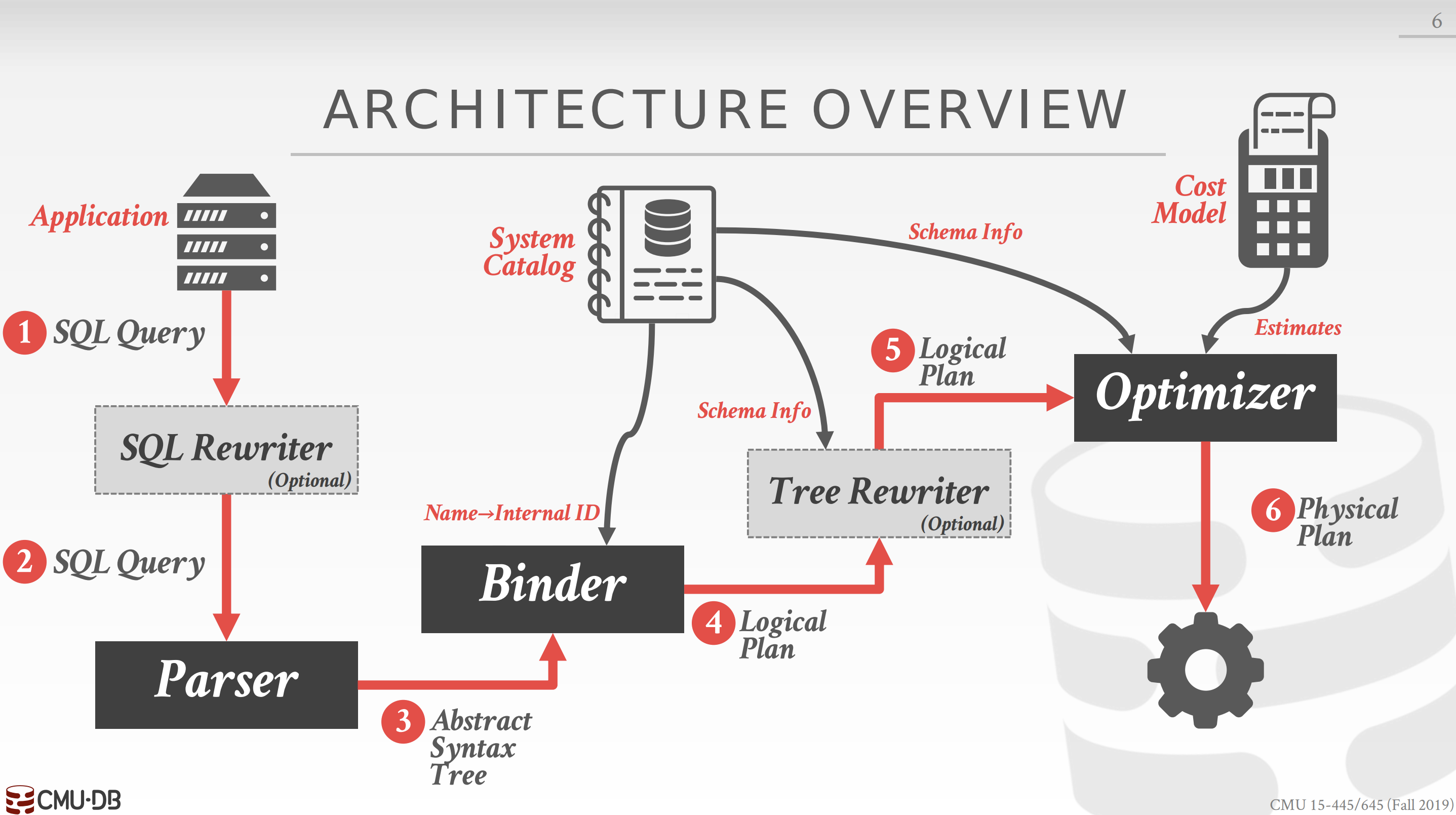
There are two types of optimization strategies:

Heuristics/Rules: Rewrite the query to remove inefficiencies. Does not require a cost model.
Cost-based Search: Use a cost model to evaluate multiple equivalent plans and pick the one with the smallest cost.

8.1 Rule-based Query Optimization

Two relational algebra expressions are equivalent if they generate the same set of tuples. Given this, the DBMS can identify better query plans without a cost model. This is technique often called query rewriting. Note that most DBMSs will rewrite the query plan and not the raw SQL string.

Examples of query rewriting:

Predicate Push-down: Perform predicate filtering before join to reduce size of join.
Projections Push-down: Perform projections early to create smaller tuples and reduce intermediate results. You can project out all attributes except the ones requested or required (e.g., join attributes).
Expression Simplification: Exploit the transitive properties of boolean logic to rewrite predicate expressions into a more simple form.

8.2 Cost-based Query Optimization

The DBMS’s optimizer will use an internal cost model to estimate the execution cost for a particular query plan. This provides an estimate to determine whether one plan is better than another without having to actually run the query (which would be slow to do for thousands of plans).

This estimate is an internal metric that (usually) is not comparable to real-world metrics, but it can be derived from estimating the usage of different resources:

**CPU:** Small cost; tough to estimate
**Disk:** Number of block transferred
**Memory:** Amount of DRAM used
**Network:** Number of messages transfered

To accomplish this, the DBMS stores internal statistics about tables, attributes, and indexes in its internal catalog. Different systems update the statistics at different times. Commercial DBMS have way more robust and accurate statistics compared to the open source systems. These are estimates and thus the cost estimates will often be inaccurate.

8.2.1 Statistics

For a relation $R$, the DBMS stores the number of tuples $(N_R)$ and distinct values per attribute $(V(A, R))$.

The selection cardinality $(SC(A, R))$ is the average number of records with a value for an attribute $A$ given $\frac{N_R}{V(A, R)}$.

Complex Predicates

The selectivity (sel) of a predicate $P$ is the fraction of tuples that qualify: $sel(A = constant) = \frac{SC(P)}{V(A, R)}$
For a range query, we can use: $sel(A \geq a) = \frac{A_{max} - a}{A_{max} - A_{min})}$.
For negations: $sel(notP) = 1 − sel(P)$.
The selectivity is the probability that a tuple will satisfy the predicate. Thus, assuming predicates are independent, then $sel(P_1 \bigvee P_2) = sel(P1) \times sel(P2)$.

Join Estimation Given a join of $R$ and $S$, the estimated size of a join on non-key attribute $A$ is approx:

$estSize \approx \frac{N_R \times N_S}{max(V(A,R), V(A,S))}$

Statistics Storage

Histograms: We assumed values were uniformly distributed. But in real databases values are not uniformly distributed, and thus maintaining a histogram is expensive. Why? just imagine you have one billiion different values under one column, each of them is 4 bytes int, then you probably need to allocate around 4GB memory for a histogram just for one column, what if you have one hundred columns? So maintaining a fine-grained histogram is expensive. We can put values into buckets (i.e., grouping the values) to reduce the size of the histograms. However, this can lead to inaccuracies as frequent values will sway the count of infrequent values. To counteract this, we can size the buckets such that their spread is the same (i.e., quantling the histogram). They each hold a similar amount of values.

Sampling: Modern DBMSs also employ sampling to estimate predicate selectivities. Randomly select and maintain a subset of tuples from a table and estimate the selectivity of the predicate by applying the predicate to the small sample.

8.2.2 Search Algorithm

The basic cost-based search algorithm for a query optimizer is the following:

Bring query in internal form into canonical form.
Generate alternative plans.
Generate costs for each plan.
Select plan with smallest cost.

It is important to pick the best access method (i.e., sequential scan, binary search, index scan) for each table accessed in the query. Simple heuristics are sometimes good enough for simple OLTP queries (i.e., queries that only access a single table). For example, queries where it easy to pick the right index to use are called sargable (Search Argument Able). Joins in OLTP queries are also almost always on foreign key relationships with small cardinality.

For multiple relation query planning, the number of alternative plans grows rapidly as number of tables joined increases. For an $n$-way join, the number of different ways to order the join operations is known as a Catalan number (approx $4^n$). This is too large of a solution space and it is infeasible for the DBMS to consider all possible plans. Thus, we need a way to reduce the search complexity. For example, in IBM’s System R, they only considered left-deep join trees. Left-deep joins allow you to pipeline data, and only need to maintain a single join table in memory.

8.2.3 Nested Sub-Queries

The DBMS treats nested sub-queries in the WHERE clause as functions that take parameters and return a single value or set of values.

Two Approaches:

Rewrite to decorrelate and/or flatten queries.
Decompose nested query and store result in sub-table.

9. Transactions

A transaction is the execution of a sequence of one or more operations (e.g., SQL queries) on a shared database to perform some higher level function. They are the basic unit of change in a DBMS. Partial transactions are not allowed.

Executing concurrent transactions in a DBMS is challenging. It is difficult to ensure correctness while also executing transactions quickly. We need formal correctness criteria:

Temporary inconsistency is allowed.
Permanent inconsistency is bad.

The scope of a transaction is only inside the database. It cannot make changes to the outside world because it cannot roll those back.

9.1 ACID

A database is a set of named data objects $(A, B, C, ..)$. A transaction is a sequence of read and write operations $(R(A), W(B))$.

The outcome of a transaction is either COMMIT or ABORT.

If *COMMIT*, all of the transaction's modifications are saved to the database.
If *ABORT*, all of the transaction's changes are undone so that it is like the transaction never happened. Aborts can be either self-inflicted or caused by the DBMS.

Correctness Criteria: ACID

Atomicity: All actions in the transaction happen, or none happen.
Consistency: If each transaction is consistent and the database is consistent at the beginning of the transaction, then the database is guaranteed to be consistent when the transaction completes.
Isolation: The execution of one transaction is isolated from that of other transactions.
Durability: If a transaction commits, then its effects on the database persist.

9.1.1 Atomicity

The DBMS guarantees that transactions are atomic. The transaction either executes all its actions or none of them.

Approach #1: Shadow Paging

DBMS makes copies of pages and transactions make changes to those copies. Only when the transaction commits is the page made visible to others.
Originally from System R but abandoned in the early 1980s. Few systems do this today (CouchDB, LMDB).

Approach #2: Logging

DBMS logs all actions so that it can undo the actions of aborted transactions.
Think of this like the black box in airplanes.
Logging is used by all modern systems for audit and efficiency reasons.

9.1.2 Consistency

The “world” represented by the database is consistent (e.g., correct). All questions (i.e., queries) that the application asks about the data will return correct results.

Approach #1: Database Consistency

The database accurately represents the real world entity it is modeling and follows integrity constraints.
Transactions in the future see the effects of transactions committed in the past inside of the database.

Approach #2: Transaction Consistency

If the database is consistent before the transaction starts, it will also be consistent after.
Ensuring transaction consistency is the application's responsibility.

9.1.3 Isolation

The DBMS provides transactions the illusion that they are running alone in the system. They do not see the effects of concurrent transactions. This is equivalent to a system where transactions are executed in serial order (i.e., one at a time). But in order to get better performance, the DBMS has to interleave the operations of concurrent transactions.

Concurrency Control

A concurrency control protocol is how the DBMS decides the proper interleaving of operations from multiple transactions.

There are two categories of concurrency control protocols:

Pessimistic: The DBMS assumes that transactions will conflict, so it doesn't let problems arise in the first place.
Optimistic: The DBMS assumes that conflicts between transactions are rare, so it chooses to deal with conflicts when they happen.

The order in which the DBMS executes operations is called an execution schedule. The goal of a concurrency control protocol is to generate an execution schedule that is is equivalent to some serial execution:

Serial Schedule: A schedule that does not interleave the actions of different transactions.
Equivalent Schedules: For any database state, the effect of executing the first schedule is identical to the effect of executing the second schedule.
Serializable Schedule: A schedule that is equivalent to some serial execution of the transactions.

When the DBMS interleaves the operations of concurrent transactions, it can create anomalies:

Read-Write Conflicts ("Unrepeatable Reads"): A transaction is not able to get the same value when reading the same object multiple times.
Write-Read Conflicts ("Dirty Reads"): A transaction sees the write effects of a different transaction before that transaction committed its changes.
Write-Write conflict ("Lost Updates"): One transaction overwrites the uncommitted data of another concurrent transaction.

There are actually two types for serializability: (1) conflict and (2) view. Neither definition allows all schedules that you would consider serializable. In practice, DBMSs support conflict serializability because it can be enforced efficiently. To allow more concurrency, some special schedules are handled at the application level.

Conflict Serializability

Schedules are equivalent to some serial schedule. This is what (almost) every DBMS supports when you ask for the SERIALIZABLE isolation level.

Schedule $S$ is conflict serializable if you are able to transform $S$ into a serial schedule by swapping consecutive non-conflicting operations of different transactions.

View Serializability

Allows for all schedules that are conflict serializable and “blind writes”. Thus allows for slightly more schedules than Conflict serializability, but difficult to enforce efficiently. This is because the DBMS does not know how the application will “interpret” values

9.1.4 Durability

All of the changes of committed transactions must be durable (i.e., persistent) after a crash or restart. The DBMS can either use logging or shadow paging to ensure that all changes are durable.

9.2 Transaction Locks

The DBMS contains a centralized lock manager that decides decisions whether a transaction can have a lock or not. It has a global view of whats going on inside the system.

Shared Lock (S-LOCK): A lock that allows multiple transactions to read the same object at the same time. If one transaction holds a shared lock, then another transaction can also acquire that same shared lock.
Exclusive Lock (X-LOCK): Allows a transaction to modify an object. This lock is not compatible for any other lock. Only one transaction can hold an exclusive lock at a time.

Executing with locks:

Transactions request locks (or upgrades) from the lock manager.
The lock manager grants or blocks requests based on what locks are currently held by other transactions.
Transactions release locks when they no longer need them.
The lock manager updates its internal lock-table and then gives locks to waiting transactions.

9.3 Two-Phase Locking Concurrency Control

Two-Phase locking (2PL) is a pessimistic concurrency control protocol that determines whether a transaction is allowed to access an object in the database on the fly. The protocol does not need to know all of the queries that a transaction will execute ahead of time.

2PL is used in most DBMSs that support transactions. The protocol automatically provides correct interleavings of transaction operations, but it requires additional steps to handle deadlocks.

The application does not typically set locks manually using SQL. The DBMS acquires the locks automatically before a query accesses or modifies an object. But sometimes the application can provide the DBMS with hints to help it improve concurrency.

Phase #1: Growing

Each transaction requests the locks that it needs from the DBMS's lock manager.
The lock manager grants/denies lock requests.

Phase #2: Shrinking

The transaction enters this phase immediately after it releases its first lock.
The transaction is allowed to only release locks that it previously acquired. It cannot acquire new locks in this phase.

On its own, 2PL is sufficient to guarantee conflict serializability. It generates schedules whose precedence graph is acyclic. But it is susceptible to cascading aborts, which is when a transaction aborts and now another transaction must be rolled back, which results in wasted work.

There are also potential schedules that are serializable but would not be allowed by 2PL (locking can limit concurrency).

9.3.1 Strong Strict Two-Phase Locking

Strong Strict 2PL (SSPL, also known as Rigorous 2PL) is a variant of 2PL where the transaction only releases locks when it finishes. A schedule is strict if a value written by a transaction is not read or overwritten by other transactions until that transaction finishes. Thus, there is not a shrinking phase in SS2PL like in regular 2PL.

The advantage of this approach is that the DBMS does not incur cascading aborts. The DBMS can also reverse the changes of an aborted transaction by just restoring original values of modified tuples.

9.3.2 2PL Deadlock Handling

A deadlock is a cycle of transactions waiting for locks to be released by each other. There are two approaches to handling deadlocks in 2PL: detection and prevention.

Approach #1: Deadlock Detection The DBMS creates a waits-for graph: Nodes are transactions, and edge from $T_i$ to $T_j$ if transaction $T_i$ is waiting for transaction $T_j$ to release a lock. The system will periodically check for cycles in waits-for graph and then make a decision on how to break it.

When the DBMS detects a deadlock, it will select a “victim” transaction to rollback to break the cycle.
The victim transaction will either restart or abort depending on how the application invoked it.
There are multiple transaction properties to consider when selecting a victim. There is no one choice that is better than others. 2PL DBMSs all do different things:

By age (newest or oldest timestamp).
By progress (least/most queries executed).
By the # of items already locked.
By the # of transactions that we have to rollback with it.
# of times a transaction has been restarted in the past.

Rollback Length: After selecting a victim transaction to abort, the DBMS can also decide on how far to rollback the transaction’s changes. Can be either the entire transaction or just enough queries to break the deadlock.

Approach #2: Deadlock Prevention When a transaction tries to acquire a lock, if that lock is currently held by another transaction, then perform some action to prevent a deadlock. Assign priorities based on timestamps (e.g., older means higher priority). These schemes guarantee no deadlocks because only one type of direction is allowed when waiting for a lock. When a transaction restarts, its (new) priority is its old timestamp.

Wait-Die ("Old waits for Young"): If $T_1$ has higher priority, $T_1$ waits for $T_2$. Otherwise $T_1$ aborts.
Wound-Wait ("Young waits for Old"): If $T_1$ has higher priority, $T_2$ aborts. Otherwise $T_1$ waits.

9.3.3 Lock Granularities

If a transaction wants to update one billion tuples, it has to ask the DBMS’s lock manager for a billion locks. This will be slow because the transaction has to take latches in the lock manager’s internal lock table data structure as it acquires/releases locks.

To avoid this overhead, the DBMS can use to use a lock hierarchy that allows a transaction to take more coarse-grained locks in the system. For example, it could acquire a single lock on the table with one billion tuples instead of one billion separate locks. When a a transaction acquires a lock for an object in this hierarchy, it implicitly acquires the locks for all its children.

Intention locks allow a higher level node to be locked in shared or exclusive mode without having to check all descendant nodes. If a node is in an intention mode, then explicit locking is being done at a lower level in the tree.

Intention-Shared (IS):Indicates explicit locking at a lower level with shared locks.
Intention-Exclusive (IX):Indicates explicit locking at a lower level with exclusive or shared locks.
Shared+Intention-Exclusive (SIX): The sub-tree rooted at that node is locked explicitly in shared mode and explicit locking is being done at a lower level with exclusive-mode locks.

9.4 Timestamp Ordering Concurrency Control

Timestamp ordering (T/O) is a optimistic class of concurrency control protocols where the DBMS assumes that transaction conflicts are rare. Instead of requiring transactions to acquire locks before they are allowed to read/write to a database object, the DBMS instead uses timestamps to determine the serializability order of transactions.

Each transaction $T_i$ is assigned a unique fixed timestamp that is monotonically increasing:

Let $TS(T_i)$ be the timestamp allocated to transaction $T_i$
Different schemes assign timestamps at different times during the transaction

If $TS(T_i) < TS(T_j)$, then the DBMS must ensure that the execution schedule is equivalent to a serial schedule where $T_i$ appears before $T_j$.

Multiple timestamp allocation implementation strategies:

System clock
Logical counter
Hybrid

9.4.1 Basic Timestamp Ordering (BASIC T/O)

Every database object $X$ is tagged with timestamp of the last transaction that successfully did read/write:

W-TS(X): Write timestamp on object X.
R-TS(X): Read timestamp on object X.

The DBMS check timestamps for every operation. If transaction tries to access an object “from the future”, then the DBMS aborts that transaction and restarts it.

Read Operations:

If $TS(T_i) < W-TS(X)$ this violates timestamp order of $T_i$ with regard to the writer of $X$. Thus you abort $T_i$ and restart it with same TS.
Else:

Allow $T_i$ to read $X$.
Update $R-TS(X)$ to $max(R-TS(X), TS(Ti))$.
Have to make a local copy of $X$ to ensure repeatable reads for $T_i$.
Last step may be skipped in lower isolation levels.

Write Operations:

If $TS(T_i) < R-TS(X)$ or $TS(T_i) < W-TS(X)$, abort and restart $T_i$.
Else:

Allow $T_i$ to write $X$ and update $W-TS(X)$ to $T_i$.
Also have to make a local copy of $X$ to ensure repeatable reads for $T_i$.

Optimization: Thomas Write Rule

If $TS(T_i) < R-TS(X)$: Abort and restart $T_i$
If $TS(T_i) < W-TS(X)$:

Thomas Write Rule: Ignore the write and allow transaction to continue.
Note that this violates timestamp order of $T_i$ but this is okay because no other transaction will ever read Ti’s write to object X.

Else: Allow $T_i$ to write $X$ and update $W-TS(X)$

The Basic T/O protocol generates a schedule that is conflict serializable if you do not use Thomas Write Rule. It cannot have deadlocks because no transaction ever waits. But there is a possibility of starvation for long transactions if short transactions keep causing conflicts.

It also permits schedules that are not recoverable. A schedule is recoverable if transactions commit only after all transactions whose changes they read or commit. Otherwise, the DBMS cannot guarantee that transactions read data that will be restored after recovering from a crash.

Potential Issues:

High overhead from copying data to transaction's workspace and from updating timestamps.
Long running transactions can get starved: The likelihood that a transaction will read something from a newer transaction increases.
Suffers from the timestamp allocation bottleneck on highly concurrent systems.

9.4.2 Optimistic Concurrency Control (OCC)

If we assume that conflicts between transactions are rare and most transactions are short lived, it may be a better approach to optimize for the common case that assumes transactions are not going to have conflicts.

OCC works well when the number of conflicts is low. This is when either all of the transactions are readonly or when transactions access disjoint subsets of data. If the database is large and the workload is not skewed, then there is a low probability of conflict, so again locking is wasteful.

The DBMS creates a private workspace for each transaction:

All modifications are applied to the workspace.
Any object read is copied into workspace.
No other transaction can read the changes made by another transaction in its private workspace.

When a transaction commits, the DBMS compares the transaction’s workspace write set to see whether it conflicts with other transactions. If there are no conflicts, the write set is installed into the “global” database

OCC Transaction Phases:

Read Phase: Track the read/write sets of transactions and store their writes in a private workspace.
Validation Phase: When a transaction commits, check whether it conflicts with other transactions.
Write Phase: If validation succeeds, apply private changes to database. Otherwise abort and restart the transaction.

Validation Phase: This is where the DBMS checks whether a transaction conflicts with other transactions. The DBMS needs to guarantee that only serializable schedules are permitted. The DBMS assigns transactions timestamps when they enter the validation phase.

$T_i$ checks other transactions for RW and WW conflicts and makes sure that all conflicts go one way (from older transactions to younger transactions). The DBMS checks the timestamp ordering of the committing transaction with all other running transactions:

If $TS(T_i) < TS(T_j)$, then one of the following three conditions must hold:

$T_i$ completes all three phases before $T_j$ begins.
$T_i$ completes before $T_j$ starts its Write phase, and $T_i$ does not write to any object read by $T_j$.
$T_i$ completes its Read phase before $T_j$ completes its Read phase, and $T_i$ does not write to any object that is either read or written by $T_j$.

Potential Issues:

High overhead for copying data locally into the transaction's private workspace.
$T_i$ completes before $T_j$ starts its Write phase, and $T_i$ does not write to any object read by $T_j$.
$T_i$ completes its Read phase before $T_j$ completes its Read phase, and $T_i$ does not write to any object that is either read or written by $T_j$.

9.4.3 Partition-Based T/O

When a transaction commits in OCC, the DBMS has check whether there is a conflict with concurrent transactions across the entire database. This is slow if we have a lot of concurrent transactions because the DBMS has to acquire latches to do all of these checks.

An alternative is to split the database up in disjoint subsets called partitions (aka shards) and then only check for conflicts between transactions that are running in the same partition.

Partitions are protected by a single lock. Transactions are assigned timestamps based on when they arrive at the DBMS. Each transaction is queued at the partitions it needs before it starts running:

The transaction acquires a partition's lock if it has the lowest timestamp in that partition's queue.
The transaction starts when it has all of the locks for all the partitions that it will access during execution.
Transactions can read/write anything that they want at the partitions that they have locked. If a transaction tries to access a partition that it does not have the lock, it is aborted + restarted.

Potential Issues:

Partition-based T/O protocol is fast if: (1) the DBMS knows what partitions the transaction needs before it starts and (2) most (if not all) transactions only need to access a single partition.
The protocol only works if (1) transactions are stored procedures (network communication causes the partition to idle because it has to wait for the next query to execute) and (2) transactions only touch one partition (multi-partition transactions cause partitions to be idle because partitions have to wait for the next query to execute).

9.5 Multi-Version Concurrency Control

Multi-Version Concurrency Control (MVCC) is a larger concept than just a concurrency control protocol. It involves all aspect of the DBMS’s design and implementation. MVCC is the most widely used scheme in DBMS. It is now used in almost every new DBMS implemented in last 10 years. Even some systems (e.g., NoSQL) that do not support multi-statement transactions use it.

The DBMS maintains multiple physical versions of a single logical object in the database.

When a transaction writes to an object, the DBMS creates a new version of that object.
When a transaction reads an object, it reads the newest version that existed when the transaction started.

The original MVCC protocol for DBMSs was first proposed in 1978 MIT PhD dissertation. The first implementation in a real DBMS was in InterBase (now open-sourced as Firebird) by Jim Starkey, who later went on to be the co-founder of NuoDB.

Key Properties

Writers don’t block the readers. Readers don’t block the writers.

Read-only transactions can read a consistent snapshot without acquiring locks. Timestamps are used to determine visibility.

Multi-versioned DBMSs can support time-travel queries that can read the database at a point-in-time snapshot.

There are four important MVCC design decisions:

Concurrency Control Protocol (T/O, OCC, 2PL, etc)
Version Storage
Garbage Collection
Index Management

9.5.1 Version Storage

This how the DBMS will store the different physical versions of a logical object.

The DBMS uses the tuple’s pointer field to create a version chain per logical tuple. This allows the DBMS to find the version that is visible to a particular transaction at runtime. Indexes always point to the head of the chain. A thread traverses chain until you find the version that is visible to you. Different storage schemes determine where/what to store for each version.

Approach #1: Append-Only Storage: New versions are appended to the same table space.

Oldest-To-Newest (O2N): Append new version to end of chain, look-ups require entire chain traversal.
Newest-To-Oldest (N2O): Head of chain is newest, look-ups are quick, but indexes need to be updated every version

Approach #2: Time-Travel Storage: Old versions are copied to separate table space.

Approach #3: Delta Storage: The original values of the modified attributes are copied into a separate delta record space.

9.5.2 Garbage Collection

The DBMS needs to remove reclaimable physical versions from the database over time.

Approach #1: Tuple Level Garbage Collection: Find old versions by examining tuples directly

Background Vacuuming: Separate threads periodically scan the table and look for reclaimable versions, works with any version storage scheme.
Cooperative Cleaning: Worker threads identify reclaimable versions as they traverse version chain. Only works with O2N.

Approach #2: Transaction Level: Each transaction keeps track of its own read/write set. When a transaction completes, the garbage collector can use that to identify what tuples to reclaim. The DBMS determines when all versions created by a finished transaction are no longer visible.

9.5.3 Index Management

All primary key (pkey) indexes always point to version chain head. How often the DBMS has to update the pkey index depends on whether the system creates new versions when a tuple is updated. If a transaction updates a pkey attribute(s), then this is treated as a DELETE followed by an INSERT.

Managing secondary indexes is more complicated:

Approach #1: Logical Pointers, Use a fixed identifier per tuple that does not change. Requires an extra indirection layer that maps the logical id to the physical location of the tuple (Primary Key vs Tuple ID).
Approach #2: Physical Pointers, Use the physical address to the version chain head.

10. Recovery

Recovery algorithms are techniques to ensure database consistency, transaction atomicity, and durability despite failures. DBMS is divided into different components based on the underlying storage device. We must also classify the different types of failures that the DBMS needs to handle.

Every recovery algorithm has two parts:

Actions during normal transaction processing to ensure that the DBMS can recover from a failure.
Actions after a failure to to recover the database to a state that ensures atomicity, consistency, and durability.

The key primitives that we are going to use in a recovery algorithm are UNDO and REDO. Not all algorithms use both of these:

UNDO: The process of removing the effects of an incomplete or aborted transaction.
REDO: The process of re-instating the effects of a committed transaction for durability.

10.1 Failure Classification

Type #1: Transaction Failures

Logical Errors: A transaction cannot complete due to some internal error condition (e.g., integrity, constraint violation)
Internal State Errors: The DBMS must terminate an active transaction due to an error condition (e.g., deadlock)

Type #2: System Failures

Software Failure: There is a problem with the DBMS implementation (e.g., uncaught divide-by-zero exception) and the system has to halt.
Hardware Failure: The computer hosting the DBMS crashes. We assume that non-volatile storage contents are not corrupted by system crash.

Type #3: Storage Media Failure

Non-Repairable Hardware Failure: A head crash or similar disk failure destroys all or parts of nonvolatile storage. Destruction is assumed to be detectable. No DBMS can recover from this. Database must be restored from archived version

10.2 Buffer Pool Management Policies

Steal Policy: Whether the DBMS allows an uncommitted transaction to overwrite the most recent committed value of an object in non-volatile storage (can a transaction write uncommitted changes to disk).

STEAL: is allowed
NO-STEAL: is not allowed

Force Policy: Whether the DBMS ensures that all updates made by a transaction are reflected on nonvolatile storage before the transaction is allowed to commit.

FORCE: Is enforced
NO-FORCE: Is not enforced

Force writes makes it easier to recover but results in poor runtime performance.

Easiest System to implement: NO-STEAL + FORCE

The DBMS never has to undo changes of an aborted transaction because the changes were not written to disk.
It also never has to redo changes of a committed transaction because all the changes are guaranteed to be written to disk at committed.
Limitation: If all of the data that a transaction needs to modify does not fit on memory, then that transaction cannot execute because the DBMS is not allowed to write out dirty pages to disk before the transaction commits.

10.3 Shadow Paging

The DBMS maintains two separate copies of the database (master, shadow). Updates are only made in the shadow copy. When a transaction commits, atomically switch the shadow to become the new master. This is an example of a NO-STEAL + FORCE system.

Implementation:

Organize the database pages in a tree structure where the root is a single disk page.
There are two copies of the tree, the master and the shadow:

The root points to the master copy
Updates are applied to the shadow copy

To install updates, overwrite the root so it points to the shadow, thereby swapping the master and shadow.

Before overwriting the root, none of the transactions updates are part of the disk-resident database
After overwriting the root, all of the transactions updates are part of the disk resident database

UNDO: Remove the shadow pages. Leave master and the DB root pointer alone
REDO: Not needed at all

10.4 Write-Ahead Logging

The DBMS records all the changes made to the database in a log file (on stable storage) before the change is made to a disk page. The log contains sufficient information to perform the necessary undo and redo actions to restore the database after a crash. This is an example of a STEAL + NO-FORCE system.

Almost every DBMS uses write-ahead logging (WAL) because it has the fastest runtime performance. But the DBMS’s recovery time with WAL is slower than shadow paging because it has to replay the log.

Implementation:

All log records pertaining to an updated page are written to non-volatile storage before the page itself is allowed to be overwritten in non-volatile storage.
A transaction is not considered committed until all its log records have been written to stable storage.
When the transaction starts, write a <BEGIN> record to the log for each transaction to mark its starting point.
When a transaction finishes, write a <COMMIT> record to the log and make sure all log records are flushed before it returns an acknowledgment to the application.
Each log entry contains information about the change to a single object:

Transaction ID.
Object ID.
Before Value (used for UNDO).
After Value (used for REDO).

Log entries to disk should be done when transaction commits. You can use group commit to batch multiple log flushes together to amortize overhead.

10.5 Checkpoints

The main problem with write-ahead logging is that the log file will grow forever. After a crash, the DBMS has to replay the entire log, which can take a long time if the log file is large. Thus, the DBMS can periodically takes a checkpoint where it flushes all buffers out to disk.

How often the DBMS should take a checkpoint depends on the application’s performance and downtime requirements. Taking a checkpoint too often causes the DBMS’s runtime performance to degrade. But waiting a long time between checkpoints can potentially be just as bad, as the system’s recovery time after a restart increases.

Blocking Checkpoint Implementation:

The DBMS stops accepting new transactions and waits for all active transactions to complete.
Flush all log records and dirty blocks currently residing in main memory to stable storage.
Write a <CHECKPOINT> entry to the log and flush to stable storage.

10.6 Logging Schemes

Physical Logging:

Record the changes made to a specific location in the database.
Example: Position of a record in a page.

Logical Logging:

Record the high level operations executed by transactions. Not necessarily restricted to single page. Requires less data written in each log record than physical logging. Difficult to implement recovery with logical logging if you have concurrent transactions in a non-deterministic concurrency control scheme.
Example: The UPDATE, DELETE, and INSERT queries invoked by a transaction.

Physiological Logging:

Hybrid approach where log records target a single page but do not specify data organization of the page.
Most commonly used approach.

Categories

Tags

1. General

1.1 Basic Terms

1.2 Relational Algebra

2. Storage Management

2.1 Database Page

2.2 Page Layout

2.3 Database Heap

2.4 Data Representation

Integers:

Variable Precision Numbers:

Fixed Point Precision Numbers

Variable Length Data

Dates and Times

2.5 Workloads

2.6 Storage Models

3. Buffer Management

3.1 Locks vs. Latches

3.2 Buffer Pool

4. Access Methods

4.1 Hash Tables

4.1.1 Hash Functions

4.1.2 Static Hashing Schemes

4.1.3 Dynamic Hashing Schemes

4.2 Tree Indexes

4.2.1 B+ Tree Introduction

4.2.2 B+ Tree Design Decisions

4.2.3 B+ Tree Optimizations

4.3 Additional Index Usage

4.3.1 Radix Tree

4.3.2 Inverted Indexes

4.4 Concurrency Control Indexes

4.4.1 Latch Implementations

4.4.2 Hash Table Latching

4.4.3 B+ Tree Latching

4.4.4 Leaf Node Scans

5. Operator Execution

5.1 Sorting

5.1.1 External Merge Sort

5.2 Aggregations

5.2.1 Sorting

5.2.2 Hashing

5.3 Join

5.3.1 Nested Loop Join

5.3.2 Sort-Merge Join

5.3.3 Hash Join

6. Query Execution

6.1 Query Plan

6.2 Processing Models

6.2.1 Iterator Model

6.2.2 Materialization Model

6.2.3 Vectorization / Batch Model

6.3 Access Methods

6.3.1 Sequential Scan

6.3.2 Index Scan

6.4 Expression Evaluation

7 Query Parallelism

7.1 Parallel DBMS vs. Distributed DBMS

7.2 Process Models

7.3 Inter-Operator Parallelism vs. Intra-Query Parallelism

7.3.1 Inter-Query Parallelism

7.3.2 Intra-Query Parallelism

7.4 I/O Parallelism

8 Query Planning & Optimization

8.1 Rule-based Query Optimization

8.2 Cost-based Query Optimization

8.2.1 Statistics

8.2.2 Search Algorithm

8.2.3 Nested Sub-Queries

9. Transactions

9.1 ACID

9.1.1 Atomicity

9.1.2 Consistency

9.1.3 Isolation

9.1.4 Durability

9.2 Transaction Locks

9.3 Two-Phase Locking Concurrency Control

9.3.1 Strong Strict Two-Phase Locking

9.3.2 2PL Deadlock Handling