Core ideas of NLP and LLM
This blog recods some core ideas of NLP (Natural Language Processing) and LLM (Large Language Model).
Word2vec or Word Embeddings
Word2vec is a method to efficiently create word embeddings, which essentially convert a token to a vector that consists of a list of numbers.
A token could be a word, a piece of words, or other common characetorer combinations. If images and sound are involved, the tokens could be little patches of that image or little chunk of that sound. Each one of these tokens is then associated with a vector, which is meant to somehow encode the meaning of that piece.
For instance, the following is a word embedding for the word king (GloVe vector trained on Wikipedia):
[0.50451, 0.68607, -0.59517, -0.022801, 0.60046, -0.13498, -0.08813, 0.47377, -0.61798, -0.31012, -0.076666, 1.493, -0.034189, -0.98173, 0.68229, 0.81722, -0.51874, -0.31503, -0.55809, 0.66421, 0.1961, -0.13495, -0.11476, -0.30344, 0.41177, -2.223, -1.0756, -1.0783, -0.34354, 0.33505, 1.9927, -0.04234, -0.64319, 0.71125, 0.49159, 0.16754, 0.34344, -0.25663, -0.8523, 0.1661 , 0.40102, 1.1685, -1.0137, -0.21585, -0.15155, 0.78321, -0.91241, -1.6106, -0.64426, -0.51042]
If we consider the embeddings for the other words such as man, woman, queen, we can have the famous equation
king - man + woman ~= queen
Continuous Bag of Words (CBOW)
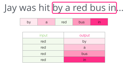
Guessing a word based on its context (the words before and after it). As shown in the following example, we want to use words “by”, “a”, “bus”, and “in” to predict red.

Therefore, the dataset we’re virtually building and training the model against would look like this:

Skipgram
Skipgram tries to guess neighboring words using the current word. We can think of the window it slides against the training text as looking like this:

In the above example, when the window slides and covers the words by a red bus in, the input is red and the predicted target words are “by”, “a”, “bus”, and “in”.
The pink boxes are in different shades because this sliding window actually creates four separate samples in our training dataset:

Recurrent Neural Network (RNN)
RNNs are networks with loops in them, allowing information to persist, sort of having memory
Humans don’t start their thinking from scratch every second. As you read this essay, you understand each word based on your understanding of previous words.
Traditional neural networks can’t do this, no historical information will be used for current event prediction. Recurrent neural networks address this issue. They are networks with loops in them, allowing information to persist.

This chain-like nature reveals that recurrent neural networks are intimately related to sequences and lists. They’re the natural architecture of neural network to use for such data.
Long Short-Term Memory (LSTM)
One of the appeals of RNNs is the idea that they might be able to connect previous information to the present task.
If we are trying to predict the last word in “the clouds are in the sky,” we don’t need any further context – it’s pretty obvious the next word is going to be sky. In such cases, where the gap between the relevant information and the place that it’s needed is small, RNNs can learn to use the past information.
However, consider trying to predict the last word in the text “I grew up in France, ……, I speak fluent French.” Recent information suggests that the next word is probably the name of a language, but if we want to narrow down which language, we need the context of France, from further back. It’s entirely possible for the gap between the relevant information and the point where it is needed to become very large.
Unfortunately, as that gap grows, RNNs become unable to learn to connect the information.
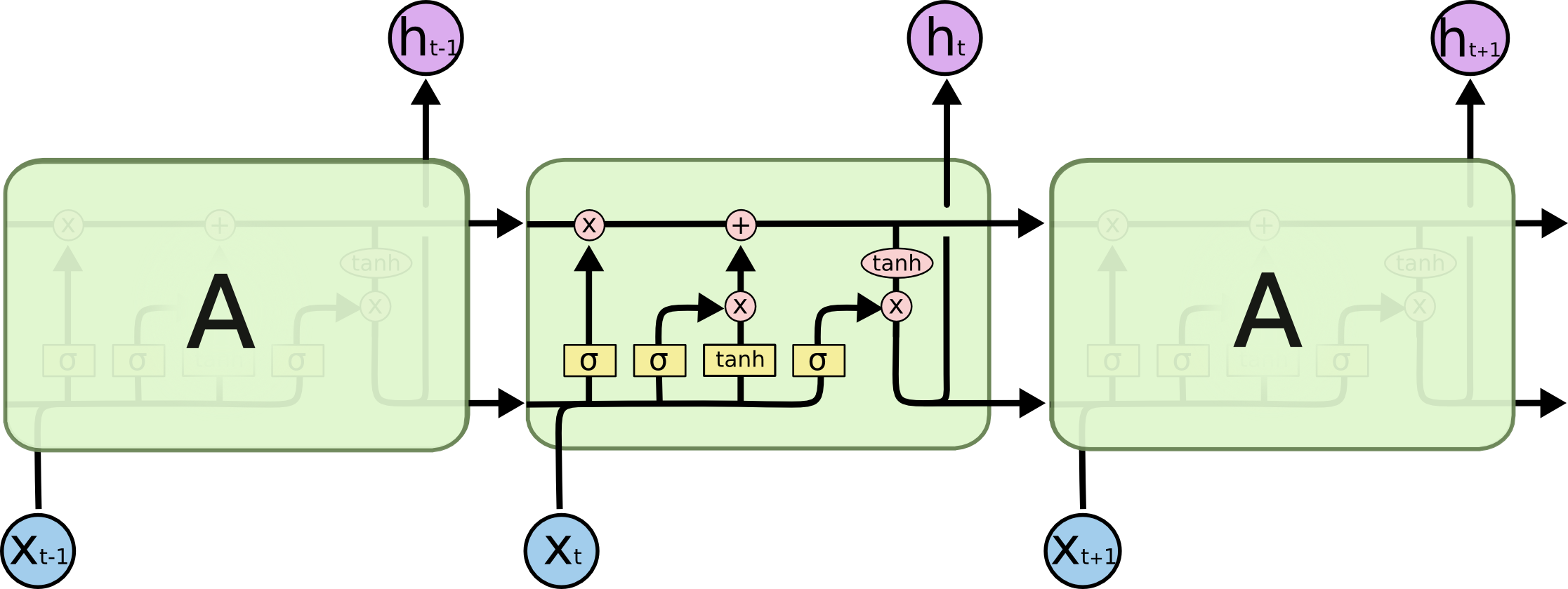
LSTMs don’t have this problem. LSTMs also have this chain like structure, but the repeating module has a different structure: there are input gate, forget gate, output gate, and a cell state.

Cell State basically encodes the information of the inputs (relevant info.) that have been observed up to that step (at every step).
The LSTM can remove or add information to the cell state, carefully regulated by structures called gates. Gates are a way to optionally let information through. They are composed out of a sigmoid neural net layer and a pointwise multiplication operation.
Therefore, when the hyperparamters of these gates (when the gate should open or close) are trained, the LSTM will know which information (even if very far away from the current context) should be persisted in the cell state which can be discarded.
Transformer
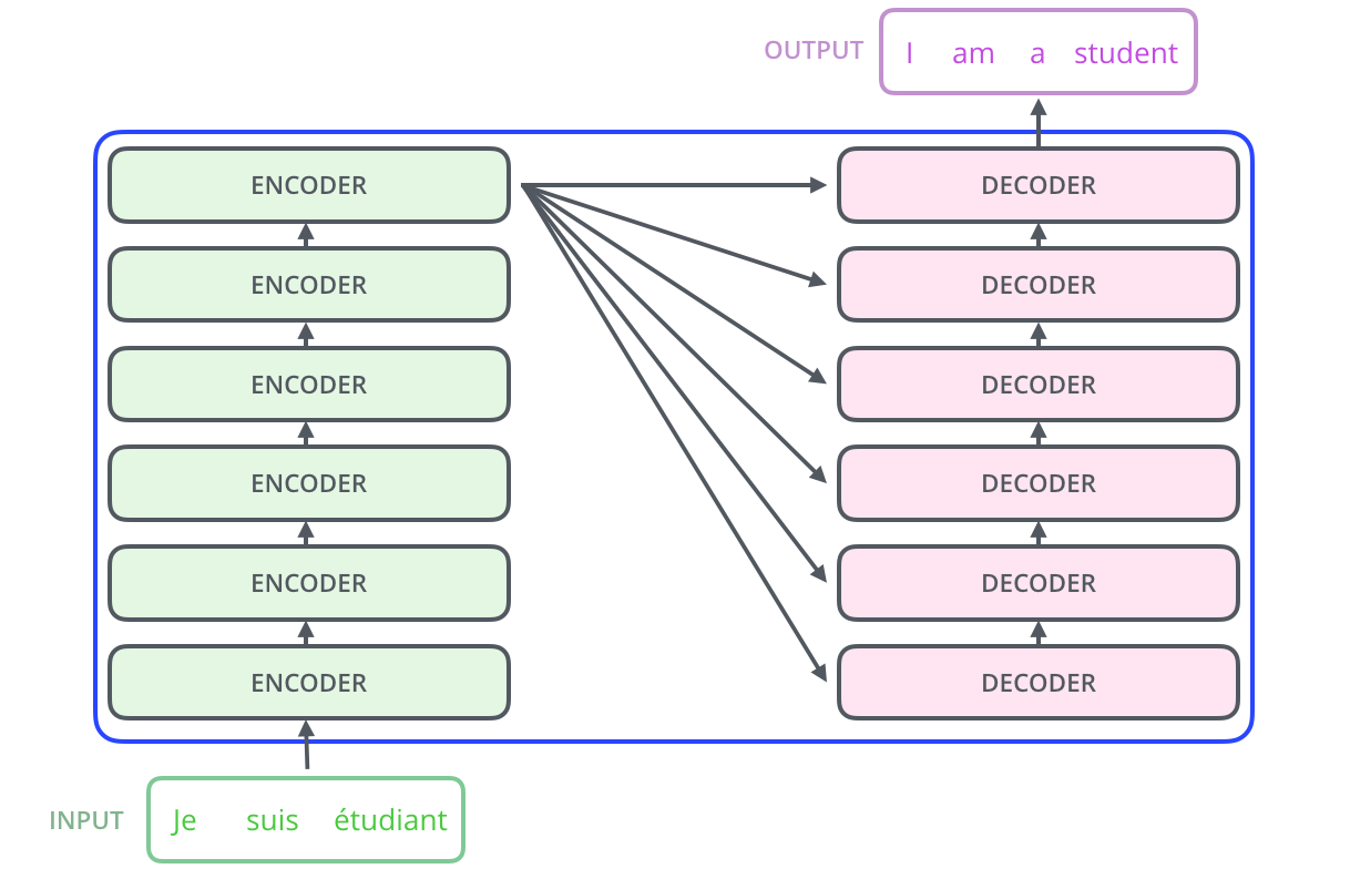
There are an encoding component, a decoding component, and connections between them in a Transformer model. The encoding component is a stack of encoders (the paper stacks six of them on top of each other, there’s nothing magical about the number six, one can definitely experiment with other arrangements). The decoding component is a stack of decoders of the same number.

The encoders are all identical in structure. Each one is broken down into two sub-layers: self-attention and feed-forward layers. The decoder has both those layers, but between them is an attention layer that helps the decoder focus on relevant parts of the input sentence.

Self-attention at a high level
As the model processes each word (each position in the input sequence), self attention allows it to look at other positions in the input sequence for clues that can help lead to a better encoding for this word. Basically, self-attention is the method the Transformer uses to bake the “understanding” of other relevant words into the one we’re currently processing. It is similar to context understanding, a word “it” may have very different meaning if we put it into different sentences (i.e., different context). So, for Transformer model, how to find the most accurate meaning of “it” is based on how the model connect “it” with other words in this sentence (or the current context).
Model Quantization
Quantization is the process of converting the weights (and activations) of a model using a lower precision. For example, weights stored using 16 bits can be converted into a 4-bit representation. This technique has become increasingly important to reduce the computational and memory costs associated with LLMs.
Large Language Model [LLM]
Retrieval Augmented Generation [RAG]
RAG is the process of optimizing the output of a large language model, so it references an authoritative knowledge base outside of its training data sources before generating a response. LLMs are trained on vast volumes of data and use billions of parameters to generate original output for tasks like answering questions, translating languages, and completing sentences. RAG extends the already powerful capabilities of LLMs to specific domains or an organization’s internal knowledge base, all without the need to retrain the model. It is a cost-effective approach to improving LLM output so it remains relevant, accurate, and useful in various contexts.
Parameter-Efficient Fine-Tuning [PEFT]
Parameter-Efficient Fine-Tuning (PEFT) enables you to fine-tune a small subset of parameters in a pretrained LLM. The main idea is that you freeze the parameters of a pre-trained LLM, add some new parameters, and fine-tune the new parameters on a new (small) training dataset. Typically, the new training data is specialized for the new task you want to fine-tune your LLM for.
Adapters add tunable layers to the various transformer blocks of an LLM. Prefix tuning adds trainable tensors to each transformer block. LoRA (Low-rank adaptation of large language models) has become a widely used technique to fine-tune LLMs. An extension, known as QLoRA, enables fine-tuning on quantized weights, such that even large models such as Llama-2 can be trained on a single GPU.
Reinforcement Learning From Human Feedback [RLHF]
RLHF is a novel approach to reducing bias in LLMs. RLHF is a usually 3-step training process.
- We start with a pre-trained LLM, and we fine-tune it with supervision (a.k.a. human feedback). Then, we will have a supervised fine-tuned (SFT) model.
- This SFT model is then used to initialize a reward model (RM) with a linear head on top. This reward model is trained with a preference dataset.
- The SFT model is again fine-tuned, but by using reinforcement learning (RL). In traditional RL, a reward function is hand-crafted, but in this case, it is the trained RM (from the previous step) as a reward function.
Datasets for fine-tune LLMs
There are different types of datasets we can use to fine-tune LLMs:
- Instruction datasets: inputs are instructions (e.g., questions) and outputs correspond to the expected responses (e.g., answers). Example: Open-Orca and Alpaca.
- Raw completion: this is a continuation of the pre-training objective (next token prediction). In this case, the trained model is not designed to be used as an assistant. Example: MADLAD-400.
- Preference datasets: these datasets are used with reinforcement learning to rank candidate responses. They can provide multiple answers to the same instruction, and help the model to select the best response. Example: ultrafeedback_binarized.
- Others: a fill-in-the-middle objective is very popular with code completion models (e.g., Codex from GitHub Copilot). Other datasets can be designed for classification, where the outputs correspond to the labels we want to predict (the model requires an additional classfication head in this case).
Reference:
- Jay Alammar - The Illustration Word2Vec: A good reference to understand the famous Word2Vec architecture.
- colah’s blog - Understanding LSTM Networks: A more theoretical article about the LSTM network.
- Parameter-Efficient Fine-Tuning (PEFT) of LLMs
- An Introduction to Training LLMs Using Reinforcement Learning From Human Feedback (RLHF)
- Dataset creation for fine-tuning LLM