Introduction to Roofline Model
The roofline model, which is created by Samuel Williams, is a visual performance model used in computer architecture and high-performance computing (HPC) to bound the performance of various numerical methods and operations running on multicore, manycore, or accelerator processor architectures.
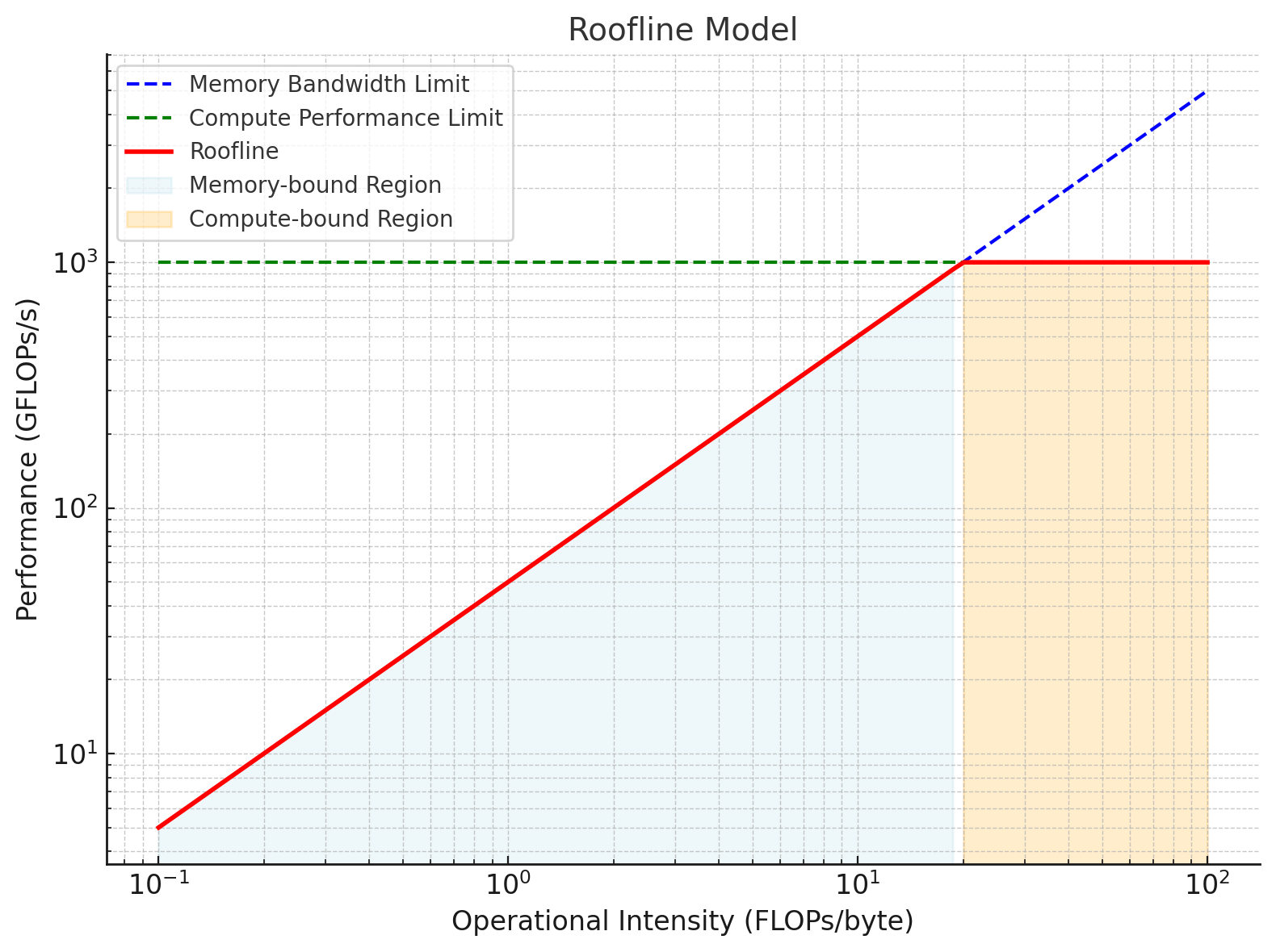
It is called the roofline model because the graph it produces looks like a roofline, with performance bounded by the system’s memory bandwidth (sloped line) and peak computational performance (flat line), as shown in the following figure[from wikipedia]:

The X-axis is Operational Intensity (GFlops per byte). The Operational Intensity is defined as the ratio of computational operations to memory traffic (FLOP/byte). It measures how much computation is performed per unit of data moved from memory.
The Y-axis is Performance or Throughput (GFlops per second). This is the most common unit and measures the speed at which a processor can perform mathematical computations–It shows how fast a program or system can execute computations.
Therefore, the roofline is defined as:
Attainable GFlops/sec = Min(Peak Floating Point Performance, Peak Memory Bandwidth x Operational Intensity)
The Peak Floating Point Performance and Peak Memory Bandwidth can be found using the hardware specifications or microbenchmarks. But what is “Operational Intensity”?
Operational Intensity
Operational Intensity measures how much computation is performed per unit of data moved from memory. Operational Intensity (OI) quantifies the efficiency of how a program uses the data it fetches from memory to do useful computational work.
Think of it as the “work-to-data” ratio:
- Work = The number of mathematical calculations (like adding, multiplying, etc.) your program performs.
- Data = The amount of information your program reads from or writes to memory. That is, we measure traffic between the caches and memory rather than between the processor and the caches.
Example
Imagine you have a program that:
- Reads 1 GB (1 billion bytes) of data from memory.
- Performs 10 billion calculations on that data.
Here, the Operational Intensity (OI) is:
$OI = \frac{\text{10 billion computations}}{\text{1 billion bytes of data moved}} = \text{10 FLOPs per byte}$
This means the program does 10 calculations for every byte it reads from memory.
- Low OI (e.g., OI = 0.5 FLOPs/byte): Most of the time is spent moving data rather than calculating.
- High OI (e.g., OI = 20 FLOPs/byte): The program efficiently uses the data it reads, doing a lot of useful work with each byte.
A low operational intensity program does very few calculations for every piece of data it loads. Example: Looking up information in a large database.
A high operational intensity program does a lot of calculations with the same piece of data. Example: Training a deep learning model, where the same weights are used repeatedly for many computations.
How to Improve Operational Intensity
Do more work with each piece of data (reuse data in faster memory like caches) and Reduce the amount of data movement (optimize your memory access patterns).
Fallacies
Fallacy: The model does not take into account all features of modern processors, such as caches or prefetching.
The definition of operational intensity considers: memory accesses are measured between the caches and memory, not between the processor and caches.
Fallacy: Doubling cache size will increase operational intensity.
Increasing cache size helps only with capacity misses and possibly conflict misses, so a larger cache can have no effect on the operational intensity.
Fallacy: The model doesn’t account for the long memory latency.
Long memory latency refers to the significant delay that occurs when a processor (CPU or GPU) has to retrieve data from the main memory (DRAM) instead of from faster, closer memory levels, such as caches. Memory latency is the time it takes for a memory request, such as reading or writing data, to be fulfilled after being issued by the processor.
The ceilings for no software prefetching are at lower memory bandwidth precisely because they cannot hide the long memory latency.
Fallacy: The model has nothing to do with multicore
Little’s Law dictates that to really push the limits of the memory system, considerable concurrency is necessary. That concurrency is more easily satisfied in a multicore than in a uniprocessor. While the bandwidth orientation of the Roofline model certainly works for uniprocessors, it is even more helpful for multicores.
Fallacy: You need to recalculate the model for every kernel
The Roofline need to be calculated for given performance metrics and computer just once, and then guide the design for any program for which that metric is the critical performance metric. The ceilings are measured once, but they can be reordered depending whether the multiplies and adds are naturally balanced or not in the kernel.
Fallacy: The Roofline model must use DRAM bandwidth.
If the working set fits in the L2 cache, the diagonal Roofline could be L2 cache bandwidth instead of DRAM bandwidth, and the operational intensity on the X-axis would be based on Flops per L2 cache byte accessed. The diagonal memory performance line would move up, and the ridge point would surely move to the left.
Reference:
- Samuel Williams, Andrew Waterman, and David Patterson. “Roofline: an insightful visual performance model for multicore architectures.” Communications of the ACM 52, no. 4 (2009): 65-76.